DISPLAYING DATA
DISPLAYING DATA. Displaying and summarising data. At the end of the session you should be able to: Understand how to appropriately display data using a variety of charts, such as stem & leaf plots, histograms, bar charts and box & whisker plots

DISPLAYING DATA
E N D
Presentation Transcript
Displaying and summarising data At the end of the session you should be able to: • Understand how to appropriately display data using a variety of charts, such as stem & leaf plots, histograms, bar charts and box & whisker plots • Understand when it is appropriate to use particular summary measures: mean, median, mode, range, interquartile range, standard deviation • Understand elementary properties of the Normal distribution • Distinguish between positive and negative skew
The scenario “Our doctor has a patient with a Haemoglobin level of 9.5. How does this compare with other people; and is this normal?”
The blood test • Haemoglobin is a compound found in red blood cells • Each molecule consists of four polypeptide chains each with its own haem group
The blood test • Blood haemoglobin is measured as a concentration • The figure usually quoted is a number of grams per deci-litre of blood (a tenth of a litre) • So our patient has a haemoglobin ‘level’ of 9.5g/dl
The blood test • People with too much haemoglobin usually have a condition known as Polycythaemia Rubra Vera. Sufferers have a ruddy complexion and may have high blood pressure, headaches and itching • People with not enough haemoglobin are said to be Anaemic. People with anaemia are pale, breathless on exertion and may suffer from chest pain
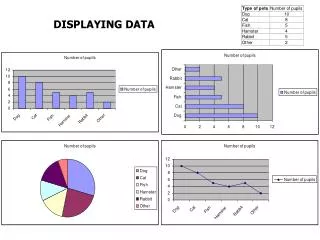
Categorical (qualitative) Nominal : no natural ordering Haemoglobin types Sex Nb: if only two categories, it is somethines called binary Ordered categorical Anaemic / borderline / not anaemic Quantitative (numerical) Count (sometimes know as discrete): can only take certain values Number of positive tests for anaemia Continuous: limited only by accuracy of instrument Haemoglobin concentration (g/dl) Types of Data
So what type of data is Haemoglobin? • Looks like haemoglobin is continuous data
The dataset • Over the past year our GP has sent off and had returned nearly 1000 blood tests • About half were for men and half were for women • Let’s consider just 50 of those results
50 randomly chosen results … numbers, numbers, numbers ... … 12.2 16.0 14.7 12.1 11.9 12.3 13.9 11.7 12.0 12.6 9.6 7.5 10.3 10.5 13.9 12.4 11.8 11.2 12.4 14.4 16.5 13.3 9.5 12.8 11.6 14.9 15.0 17.8 12.8 11.1 11.0 10.7 15.3 15.8 13.9 10.5 5.1 14.6 13.3 10.4 12.6 12.1 15.0 15.4 11.6 9.3 10.8 12.7 12.2 13.1
50 randomly chosen results … numbers, numbers, numbers ... … 12.2 16.0 14.7 12.1 11.9 12.3 13.9 11.7 12.0 12.6 9.6 7.5 10.3 10.5 13.9 12.4 11.8 11.2 12.4 14.4 16.5 13.3 9.5 12.8 11.6 14.9 15.0 17.8 12.8 11.1 11.0 10.7 15.3 15.8 13.9 10.5 5.1 14.6 13.3 10.4 12.6 12.1 15.0 15.4 11.6 9.3 10.8 12.7 12.2 13.1
Blood data: a stem & leaf plotstem – Whole g/dl leaf – 0.1g/dl Frequency Stem & Leaf .00 7 . .00 8 . .00 9 . .00 10 . .00 11 . 1.00 12 . 2 .00 13 . .00 14 . .00 15 . .00 16 . .00 17 . Stem width: 1.00 Each leaf: 1 case(s)
50 randomly chosen results … numbers, numbers, numbers ... … 12.2 16.0 14.7 12.1 11.9 12.3 13.9 11.7 12.0 12.6 9.6 7.5 10.3 10.5 13.9 12.4 11.8 11.2 12.4 14.4 16.5 13.3 9.5 12.8 11.6 14.9 15.0 17.8 12.8 11.1 11.0 10.7 15.3 15.8 13.9 10.5 5.1 14.6 13.3 10.4 12.6 12.1 15.0 15.4 11.6 9.3 10.8 12.7 12.2 13.1
Blood data: a stem & leaf plotstem – Whole g/dl leaf – 0.1g/dl Frequency Stem & Leaf .00 7 . .00 8 . .00 9 . .00 10 . .00 11 . 1.00 12 . 2 .00 13 . .00 14 . .00 15 . 1.00 16 . 0 .00 17 . Stem width: 1.00 Each leaf: 1 case(s)
50 randomly chosen results … numbers, numbers, numbers ... … 12.2 16.014.7 12.1 11.9 12.3 13.9 11.7 12.0 12.6 9.6 7.5 10.3 10.5 13.9 12.4 11.8 11.2 12.4 14.4 16.5 13.3 9.5 12.8 11.6 14.9 15.0 17.8 12.8 11.1 11.0 10.7 15.3 15.8 13.9 10.5 5.1 14.6 13.3 10.4 12.6 12.1 15.0 15.4 11.6 9.3 10.8 12.7 12.2 13.1
Blood data: a stem & leaf plotstem – Whole g/dl leaf – 0.1g/dl Frequency Stem & Leaf .00 7 . .00 8 . .00 9 . .00 10 . .00 11 . 1.00 12 . 2 .00 13 . 1.00 14 . 7 .00 15 . 1.00 16 . 0 .00 17 . Stem width: 1.00 Each leaf: 1 case(s)
Blood data: a stem & leaf plotstem – Whole g/dl leaf – 0.1g/dl Frequency Stem & Leaf 1.00 Extremes (=<5.1) 1.00 7 . 5 .00 8 . 3.00 9 . 356 6.00 10 . 345578 8.00 11 . 01266789 13.00 12 . 0112234466788 6.00 13 . 133999 4.00 14 . 4679 5.00 15 . 00348 2.00 16 . 05 1.00 17 . 8 Stem width: 1.00 Each leaf: 1 case(s)
Blood data: a histogram Patient value
Displaying nominal data • Can use either bar charts or pie charts • Display percentages, not proportions • Always give sample sizes • Avoid 3-D charts • Only use pie charts when the number of categories is low (< 5)
For example….. • Suppose that we suspect that there may be sex differences in Hb • Let’s look at the percentage of our total sample (991 people) with Hb less than 9.5g/dl, by sex ……………….
Blood data: a bar chart Bar chart showing percentage of blood results under 9.5g/dl by sex (n=67) Percentage of cases (%)
Blood data: a bar chart Bar chart showing percentage of blood results under 9.5g/dl by sex (n=67) Percentage of cases (%) Percentage of cases (%) Figure 2: 3-D bar chart (not recommended) Figure1: 2-D bar chart (recommended)
Blood data: a pie chart Pie chart showing percentage of blood results under 9.5g/dl by gender (n=67)
Slide of data for the 991 observations 15.1 10.0 22.7 14.5 14.4 15.1 13.0 8.4 12.2 10.3 9.0 16.0 12.7 9.5 10.9 15.2 12.7 11.7 11.9 14.7 13.9 15.0 13.6 7.3 13.2 14.2 12.9 11.8 12.1 15.1 13.0 11.5 11.7 11.6 10.5 8.1 11.0 11.0 9.4 8.9 15.8 17.1 17.4 12.4 11.1 10.0 12.6 14.0 12.4 11.8 10.9 10.4 12.8 12.4 11.6 10.9 15.2 7.2 8.6 10.8 13.9 16.6 14.8 12.9 11.6 12.6 12.7 17.0 15.8 16.0 13.0 11.9 12.5 14.1 12.9 16.0 10.2 7.2 12.3 12.3 14.1 11.6 12.9 14.7 14.9 15.6 12.8 16.0 16.1 12.0 11.4 15.8 9.7 13.0 11.6 12.3 11.5 10.0 15.0 9.9 14.3 14.0 15.4 11.5 11.9 13.9 12.4 11.0 13.3 13.0 10.0 10.7 15.6 15.3 16.8 12.3 13.9 14.1 11.2 8.3 13.5 11.8 8.8 9.0 12.1 11.7 10.6 14.8 13.1 14.8 12.5 15.4 12.3 16.4 16.0 10.6 10.5 12.0 12.9 12.2 12.4 16.2 15.6 15.7 12.6 9.6 13.3 9.5 10.1 11.0 15.8 14.2 12.5 14.3 15.9 14.1 10.7 18.1 14.6 13.8 15.8 10.7 8.7 12.9 7.6 5.7 12.2 9.9 10.4 9.9 7.5 12.4 10.3 10.5 13.9 10.1 17.7 12.4 11.5 11.8 10.5 13.3 12.4 14.3 15.4 15.5 13.3 13.4 12.0 14.4 16.0 15.4 10.1 13.0 14.5 15.1 15.9 15.8 14.6 14.0 14.0 15.9 14.5 14.4 13.4 9.3 13.5 21.1 12.4 12.1 9.2 11.6 10.4 11.4 11.9 8.5 8.6 9.2 13.9 15.8 11.6 16.8 14.1 13.0 13.2 10.7 14.0 15.9 14.9 14.3 14.6 13.7 13.6 14.6 14.9 15.2 16.1 14.3 14.8 14.2 14.5 14.8 15.2 10.5 11.1 16.5 15.2 15.7 15.7 14.2 12.5 10.1 14.4 12.3 10.0 9.5 14.3 15.4 14.6 12.2 11.7 11.2 14.3 15.0 14.4 14.7 14.5 16.4 12.3 12.9 14.3 15.8 12.8 13.4 12.8 15.3 12.7 11.9 12.6 12.1 15.2 14.1 15.3 14.7 15.2 14.3 11.6 13.9 14.2 14.9 12.6 10.5 10.7 15.4 14.4 15.8 13.3 11.4 13.0 13.1 15.6 12.0 14.8 14.9 16.2 12.8 14.8 13.5 15.7 12.7 6.2 17.7 14.8 10.2 14.3 10.6 16.7 15.5 14.6 16.0 15.5 12.1 10.7 11.9 15.8 13.1 20.4 12.8 13.6 14.0 12.9 13.3 14.9 12.7 8.5 15.0 17.8 10.6 12.0 8.8 12.8 9.9 11.4 13.2 11.3 9.6 12.1 8.5 11.8 10.1 10.9 9.0 10.5 15.8 15.1 15.7 11.1 14.9 9.3 14.5 14.7 15.2 11.5 14.8 11.5 12.9 12.6 14.9 13.1 11.1 13.5 12.9 11.6 10.4 15.2 13.2 11.8 10.1 13.2 9.5 11.5 11.5 11.5 7.9 13.9 10.1 12.9 11.0 9.8 12.2 10.7 10.1 11.1 13.5 13.4 10.3 13.1 15.1 15.5 17.9 8.1 7.8 13.6 15.7 10.8 15.5 11.4 15.7 15.5 12.7 11.6 12.7 12.5 15.3 11.4 8.5 10.4 15.4 15.6 11.0 14.3 8.9 12.4 15.5 15.8 8.8 14.0 11.1 14.0 11.8 13.9 11.8 11.9 10.6 10.7 17.2 13.0 12.3 14.8 12.6 16.7 9.2 13.3 13.0 14.0 14.4 14.2 10.8 12.2 11.9 10.0 14.0 12.4 10.2 7.4 12.9 11.8 12.6 8.9 13.7 13.3 11.7 8.5 10.8 10.2 12.4 10.5 14.1 14.6 10.5 9.7 13.8 13.1 11.8 15.3 12.3 14.7 10.8 13.3 9.3 12.9 16.0 14.8 15.8 10.5 10.0 15.0 12.9 15.1 13.3 16.0 10.7 15.7 12.6 15.7 7.4 11.4 9.2 5.1 10.1 12.8 11.9 12.8 13.2 11.9 10.9 14.1 12.9 14.2 11.5 11.5 13.6 10.1 13.8 12.4 11.7 12.1 10.5 11.6 11.8 11.1 10.0 11.8 12.2 12.4 11.7 11.2 13.2 9.8 13.5 12.3 11.1 11.6 12.7 13.9 11.8 11.2 10.9 10.1 11.2 10.8 12.8 11.9 10.1 13.8 11.2 11.3 10.0 13.9 12.0 6.9 14.0 12.3 9.9 10.6 10.4 12.6 11.3 10.8 13.0 14.9 14.0 13.0 13.0 11.2 14.2 13.1 11.1 12.7 13.9 13.4 15.4 16.0 11.3 12.1 9.3 6.6 10.0 13.0 10.8 12.6 13.0 10.6 14.9 10.1 11.4 13.2 14.0 12.2 8.1 10.9 10.2 13.4 8.6 12.9 12.7 14.8 8.9 10.2 12.9 14.6 14.0 13.8 9.9 13.4 12.0 8.1 10.4 8.8 14.0 10.6 11.9 7.9 12.5 12.4 14.1 9.6 13.0 12.5 11.3 13.3 13.1 12.8 13.3 12.1 9.9 12.4 11.2 12.3 12.1 13.2 12.8 13.9 12.4 12.4 11.7 10.4 13.2 11.0 12.0 10.6 11.6 13.1 9.4 10.2 9.7 13.0 9.7 15.3 13.5 14.8 14.3 12.8 14.8 15.1 13.4 12.6 10.8 13.0 21.6 14.9 11.0 8.1 9.8 12.7 13.1 12.0 12.6 14.2 12.3 10.4 13.7 12.5 12.1 8.7 14.9 13.4 9.9 10.7 13.9 13.1 11.5 11.4 10.3 12.2 11.2 11.9 14.4 12.9 13.7 10.8 13.4 12.6 10.3 13.7 11.6 12.5 12.7 13.4 13.7 13.1 11.0 11.6 12.6 11.8 12.3 12.1 11.6 13.1 12.1 13.5 12.7 12.3 13.4 11.1 14.0 8.7 12.7 14.2 14.3 12.9 14.8 13.2 12.7 15.3 10.7 14.0 14.0 13.2 14.2 12.7 9.2 13.1 11.2 13.2 13.2 14.6 15.9 13.1 13.1 12.4 12.3 12.0 12.9 11.1 12.2 10.2 9.6 10.1 13.0 10.2 11.5 12.3 8.9 10.7 11.9 11.2 12.0 12.2 10.9 11.0 11.1 9.9 11.7 10.9 12.4 11.6 11.0 11.6 11.1 12.7 12.6 12.0 11.7 12.5 13.1 12.6 10.9 11.8 12.6 9.8 15.0 14.5 13.6 11.1 7.5 13.7 15.1 12.1 11.4 13.7 11.5 15.4 13.7 12.2 11.6 10.4 12.2 12.8 13.1 11.8 12.4 12.6 14.0 12.8 14.6 13.0 13.2 11.2 14.6 13.1 10.6 12.2 14.1 10.9 9.3 14.4 12.6 12.1 12.7 12.0 12.9 12.5 12.7 9.7 9.1 14.1 13.8 11.9 14.7 11.1 12.4 10.5 12.6 12.1 12.1 12.0 13.2 12.7 13.7 13.5 10.5 12.2 11.4 13.7 14.8 12.9 13.8 14.7 13.8 14.6 8.4 12.4 12.4 13.4 12.6 10.8 11.7 12.7 14.0 11.7 12.2 14.5 12.6 14.3 13.1 13.4 14.5 12.5 10.8 14.0 8.1 11.0 10.7 8.4 12.4 13.8 13.1 13.7 12.6 13.2 11.8 12.9 13.0 12.7 14.1 14.8 12.9 14.3 12.7 13.0 13.6 13.2 10.0 11.8 15.3 15.6 13.4 12.0 14.1 14.2 13.1 13.7 10.8 10.6 13.1 12.9 14.0 9.4 10.7 9.5 14.3 13.7 10.3 13.4 10.7 11.2 9.6 12.6 9.5 13.7 12.3 13.3 10.2 13.3 12.8 12.4 12.6 11.1 14.3 14.5 12.7 12.9 15.4 14.6 11.6 13.2 14.0 12.9 11.0 14.2 10.1 11.2 11.2 12.8 13.0 10.9 11.7 13.9 6.4 13.0 10.2 14.3 13.1 11.7 14.2 14.6 13.8 12.8 14.8 10.6 11.8 14.9 14.2 11.6 8.2 13.1 9.8 12.4 12.3 16.3 11.5 14.1 12.2 11.4 6.9 11.3 12.1 11.4 8.3 9.8 9.7 10.0 9.9 11.3 11.9 15.7 13.1 12.2 13.7 10.0
And so what can we do with these numbers? • Can summarise them by examining some measure of their ‘middle value’ or location Additionally: • Can summarise them by examining their spread But how do we do this…..?
Measures of location Mode Most common observation Median Middle observation, when the data are arranged in order of increasing value If have even number of observations, e.g. if we take 50 results, the midpoint falls between the 25th and 26th, the median is calculated as the average of the two middle observations. Mean Sum of all observations Number of observations
For our data (991 blood results in all) Mode = 12.4 g/dl Median = 12.6 g/dl Mean 12435.5 = 12.55 g/dl 991 Our patient has a value that is lower than all of these statistics… might they be anaemic?
Pros and cons of mean/ median/ mode • Median robust to outliers (the mean is not). • Median/mode reflects what ‘most’ people experience. • Median useful when the distribution is skewed. • Mean uses all the data (more ‘efficient’). • Mean is ‘expected’ value. • Mean more common with statistical tests. • Mode rarely used, but can be useful for grouped or categorical data.
Measures of spread Range minimum observation to maximum observation Interquartile range observation below which the bottom 25% of data lie and the observation above which the top 25% of data lie NB: If value falls between two observations, eg if 25th centile falls between 5th and 6th observations then the value is calculated as the average of the two observations (this is the same principle as for the median). Standard deviation (SD) Average distance of the observations from the mean value ( NB: Variance = SD squared)
Box & whisker plot/box plots for comparing the distribution of continuous data across several groups • The box illustrates the interquartile range and thus contains the middle 50% of the data. • The median is shown by the horizontal line across the box. • The whiskers extend to the largest & smallest values excluding the outlying values. The outlying values are those values more than 1.5 box lengths from the upper or lower edges. Those observations between 1.5 and 3 box lengths from upper or lower edges of the box are outliers, whilst those more than 3 box lengths away are called extreme values. • Very useful when comparing several sets of data.
And back to our sample of 991 observations • Our sample mean Hb is 12.55g/dl • And our sample standard deviation is 2.12g/dl • So our result of 9.5 is more than one SD away from the mean… ….but what does this mean?
The Normal distribution • Bell shaped and symmetrical. • 68% of the observations lie within 1 SD of the mean. • About 95% of the observations lie within 2 SDs of the mean. • Mean and median will coincide.
Histogram of Haemoglobin concentration (g/dl), for all 991 observations
Haemoglobin concentration data Figure 1: males (n=495) Figure 2: females (n=496) Percentage (%) Percentage (%) Haemoglobin concentration (g/dl) Haemoglobin concentration (g/dl)
The dataset • So it seems that women tend to have a lower Haemoglobin than men (male mean=12.9, female mean=12.2) • But regardless of our patient’s gender 9.5g/dl seems to be a low result • The spread for females is less- why might this be? • Of course our dataset was only looking at people having their blood taken- and these might be expected to be more ill than the average population!
Is Haemoglobin data Normally distributed? • The sample Haemoglobin data show a remarkably good fit or agreement with the theoretical statistical model based on the Normal distribution (overall and for males and females separately). • This is not unusual and many other clinical measurements such as height,blood pressure,biochemical measures, tend to follow a Normal distribution in the general population.
Reference or normal ranges from our sample data • We can use the fact that our sample Haemoglobin data appear Normally distributed to calculate a reference range. • We have already mentioned that about 95% of the observations (from a Normal distribution) lie within approximately 2SDs of the mean. • So a reference range for our sample is: • Male: 12.9 (2 x 2.4) = 8.1 to 17.7 g/dl • Females: 12.2 (2 x 1.8) = 8.6 to 15.8 g/dl
Reference ranges for non-Normally distributed data • If the data are not Normally distributed then we can base the normal reference range on the observed percentiles of the sample (empirical normal range). • I.e. 95% of the observed data lie between the 2.5 and 97.5 percentiles. • So a percentile-based reference range for our sample is: • Male: 8.2 to 16.9 g/dl • Females: 8.1 to 15.2 g/dl • Most clinical reference ranges are based on samples larger than 500 people and usually on healthy subjects…………..
Normal Haemoglobin ranges • Over many years, labs have collected results from millions of ‘healthy’ people and come up with a normal Haemoglobin range for men and women. • These ranges represent results that are acceptable in patients. • For men it is a range of 13.5-17.5 g/dl • For women the range is 11.5-15.5 g/dl
Haemoglobin (g/dl), males Reference range Patient Percentage (%) Haemoglobin (g/dl)
Normal ranges • So our patient’s result is low and appears to suggest they have anaemia • Further tests would be required to identify the cause- internal bleeding, abnormal blood cell production or rapid cell destruction (perhaps due to a heart valve) • Whatever we decide to do we’re sure this patient’s blood result isn’t normal: even if the distribution of blood results is!
Session recap At the end of the session you should be able to: • Display data using stem & leaf plots, histograms, bar charts and box & whisker plots • Calculate the summary measures: mean, median, mode, range, interquartile range, standard deviation • Understand elementary properties of the Normal distribution • Distinguish between positive and negative skew
Next week…….. • In the next “Critical numbers” session we are going to look at sampling and confidence intervals.
Formula for the mean : mean (x-bar) : Greek capital letter sigma for the summation symbol, sum values from i=1 to n xi: observation i n: number of observations
Variance The variance (usually abbreviated to var, s2, or 2) is defined as: n 2 å x - x ) ( i = Var = s2 = i 1 n - 1 The units of variance are the original units squared e.g. g/dl2 for Haemoglobin. Therefore we usually use……
Standard deviation The standard deviation (usually abbreviated to SD, s, or ) is defined as the square root of the variance: n 2 å - ( x ) x i = = i 1 s - n 1