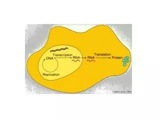
A Typical Eukaryotic Pre-mRNA Structure:
A Typical Eukaryotic Pre-mRNA Structure:. What is alternative splicing?. Exon 2. Exon 3. Exon 4. Exon 5. Exon 1. pre-mRNA of fibronectin. Intron 1. Exon 2. Intron 2. Exon 3. Exon 4. Exon 5. Exon 1. Alternative splicing. Exon 3. Exon 5. Exon 1. Mature mRNA in Firoblast cell.

A Typical Eukaryotic Pre-mRNA Structure:
E N D
Presentation Transcript
Exon 2 Exon 3 Exon 4 Exon 5 Exon 1 pre-mRNA of fibronectin Intron 1 Exon 2 Intron 2 Exon 3 Exon 4 Exon 5 Exon 1 Alternative splicing Exon 3 Exon 5 Exon 1 Mature mRNA in Firoblast cell Mature mRNA in Hepatocyte cell
A few facts about alternative splicing in human genome: • Many alternatively spliced mRNAs may be expressed • simultaneously in the same tissue. • 30-60% of genes undergo alternative splicing. • But the presence of multiple alternatively spliced mRNA • forms is not addressed in microarray design and analysis.
Known Gene Structure information: 21 well characterized genes Design a special chip of splicing variants Statistical Modeling for assessing the amounts of Splicing variants
Idea: Concentration of features containing the probes Intensities of Specially designed probes Amounts of the Individual splicing variants Features are exons or exon-exon junctions Gene Structure specifies the features of each alternative Splicing variant (or form).
Statistical Modeling: Splicing variants Features Mapped to Mapped to Probe
Relationship between features and splicing variants (or forms, transcripts): G is qx t matrix: rows: q features columns: tsplicing variants entry glk is 1 or 0 1 means presence of lfeature in k variant (or transcript) 0 means absence of l feature in k variant (or transcript) Relationship between splicing variants (or forms, transcripts) and samples (or experiments): T is t x x matrix: rows: t splicing variants columns: x samples entry tkj is the concentration of variant kin samplej variant samples features variant
C is a q x x matrix with the entry cljrepresenting the concentration of feature l in sample j samples features Next, Capture the relationship between the probes and features with Matrix F F = (fil) is a p x q matrix with values 0 or 1. fil = 1 if probepair i belongs to feature l 0 otherwise features Probe pairs
In matrix X, the entry xijrepresents the actual concentration of all the target variants (or transcripts) in sample j interrogated by probe pair i samples Probe pairs
Question: how to relate X to the matrix Y of observed probe pair intensity differences (PM-MM)? samples Probe pairs
Affinity matrix A for probe pairs, like that in Li and Wong’s model: A =(aii)is a p x p diagonal matrix where aiirepresents the affinity term of probe pair i.
With random error Obtain the model estimates for A and T by least square: A: affinity terms for probe pairs T: The amounts of splicing variants in samples
Model validation with experiment: • Dilution experiments to test the accuracy and • sensitivity. • Two-variant spike experiments: • genes like CD44 have two splice variants • Three sets: • Set 1: first variant ranges from 0 to 64 pM • second variant ranges from 64 to 0 pM • the two variants mixed and the total Concentration held at 64 pM. • Set 2: set 1 diluted 4 times, and the total concentration reached 16 pM • Set 3: Set 1 diluted 16 times, and the total concentration reached 16 pM
Three-variant spike experiments: A third CD44 variant added Designed to test all possible combinations of clones at 0 and 4 pM
Tissue experiments with TPM2 gene: Two variants: TPM2-A, containing exon A, mainly present in skeletal muscle TPM2-B, containing exon B, in esophagus, stomach, uterus, etc TagMan experiment is done for validation. Microarray experiment TaqMan Experiment