Read : Ch. 17 in Electric Circuits, 9 th Edition by Nilsson

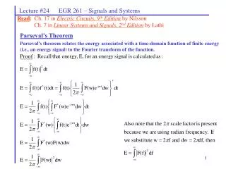
1. Lecture #24 EGR 261 – Signals and Systems Read: Ch. 17 in Electric Circuits, 9th Edition by Nilsson Ch. 7 in Linear Systems and Signals, 2nd Edition by Lathi Parseval’s Theorem Parseval’s theorem relates the energy associated with a time-domain function of finite energy (i.e., an energy signal) to the Fourier transform of the function.

2. Lecture #24 EGR 261 – Signals and Systems Parseval’s Theorem Energy calculated in the time domain Energy calculated in the frequency domain Example: Calculate total energy for the function f(t) = e-atu(t) a) In the time domain b) In the frequency domain

3. Lecture #24 EGR 261 – Signals and Systems • Notes on Parseval’s theorem: • For real functions, f(t), |F(w)| is even and F*(w) = F(-w), so: • Recall that our definition for energy is not dimensionally correct. However, if f(t) = v(t) or i(t) then the energy could be viewed as energy for a 1Ω load as shown below: • Parseval’s theorem gives a physical interpretation of |F(w)|2: • |F(w)|2 is an energy density in joules per hertz (to a 1Ω load) • Illustration: |F(w)|2 Energy = 10(8) = 80 J Note: 10 J/Hz Area under |F(w)|2 w (rad/s) -4 4

4. Lecture #24 EGR 261 – Signals and Systems Notes on Parseval’s theorem: Energy of the frequency range (w1, w2) can be calculated as follows:

5. LM 3dB B = w2 - w1 w (rad/s) w1 w2 F(w) F(w) B w w -B 0 B Essential B Lecture #24 EGR 261 – Signals and Systems Bandwidth of a filter: Recall in our earlier discussions of band pass filters, that we defined the bandwidth B of a filter as the width of the passband, typically defined by the 3dB points, as illustrated below. Bandwidth of a signal: Suppose that now we define the bandwidth of a signal as positive range of frequency over which F(w) extends, as illustrated below on the left. For any practical signal, F(w) extends to , so a practical estimate of bandwidth might be the range where most (perhaps 95%?) of the signal energy lies. This is sometimes called the essential bandwidth of the signal.

6. Lecture #24 EGR 261 – Signals and Systems • Example: If f(t) = i(t) = 50e-10tu(t) mA is the current delivered to a 1 Ω resistor: • a) Find total energy in the time domain • Find total energy in the frequency domain • Find the percentage of energy for |w| < 10 rad/s • Find the bandwidth, B, of the signal (i.e., the value of w such that 95% of the energy is delivered from 0 to |w|) • Sketch |F(w)|2 and the results from parts c and d.

7. |F(w)|2 Most of the signal energy is contained in the first lobe, so B ≈2π/ rad/s = 1/  Hz f(t) = rect(t/) 1 w -6π/ -4π/ -2π/ 2π/ 4π/ 6π/ 0 t -/2 0 /2 Lecture #24 EGR 261 – Signals and Systems Bandwidth of sinc(x): Recall that the function rect(t/) is an important function and has the following Fourier transform:

8. Lecture #24 EGR 261 – Signals and Systems Bandwidth of sinc(x): Using the result that the essential bandwidth is approximately 1/ for a gated pulse of width : The relationships above are illustrated on the following page.

9. f(t) = (t) |F(w)|2 t w 0 |F(w)|2 f(t) = rect(t/1us) 1 1us t w 0 0 -2πM 2πM |F(w)|2 f(t) = rect(t/1ms) 1 t w 0 0 -2πk 2πk -0.5ms 0.5ms |F(w)|2 f(t) = rect(t/1) 1 t w 0 -2π 2π 0 -0.5s 0.5s |F(w)|2 = [2π(w)]2 f(t) = 1 t w 0 0 Lecture #24 EGR 261 – Signals and Systems B =  B B = 1 MHz B = 2 Mrad/s B B = 1 kHz B = 2 krad/s B B = 1 Hz B = 2 rad/s B = 0