The Normal Model
This lesson focuses on the Normal distribution and the importance of checking the Nearly Normal Condition for data modeling. The distribution should be roughly unimodal and symmetric, which can be visually assessed through histograms or normal probability plots. The presentation covers the essentials of Standard Scores (z-scores) and the empirical 68-95-99.7 rule. Using an example of fuel efficiency in vehicles, we will estimate percentages of cars with certain mpg ratings and explore the characteristics of the overall distribution, emphasizing the model's application in real data scenarios.


The Normal Model
E N D
Presentation Transcript
The Normal Model Ch. 6
Approximating with the Normal model Nearly Normal Condition • The shape of the data’s distribution is roughly unimodal and symmetric. • Check this by making a histogram (or Normal probability plot) • YOU MUST CHECK THE NEARLY NORMAL CONDITION!!!
“All models are wrong – but some are useful.” -- George Box
Statistics vs. Parameters Statistics Parameters Values that specify the model -- mean -- standard deviation N(, )—Normal model with mean and standard deviation • Summaries of actual data
Rescale the Data • Standardize the data so that the: • average is 0 • standard deviation is 1 • Convert the data to z-scores • Each value is converted to a Standard Score (z-score)
The Normal Model - 1 - 2 - 3 + 1 + 2 + 3
The 68-95-99.7 Rulea.k.a. The Empirical Rule 68% 95% 99.7% - 1 - 2 - 3 + 1 + 2 + 3
The Setup The distribution of fuel efficiency of a particular vehicle is roughly unimodal and symmetric with mean 24 mpg and standard deviation 6 mpg.
Check the Nearly Normal Condition • Sketch the Normal model • What percent of all cars get less than 15 mpg? • Describe the fuel efficiency of the worst 20% of all cars. • What percent of all cars get between 20 mpg and 30 mpg? • What percent of cars get more than 40 mpg? • What gas mileage represents the third quartile? • Describe the gas mileage of the most efficient 5% of all cars.