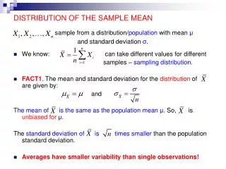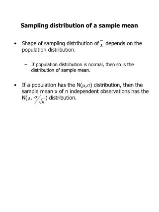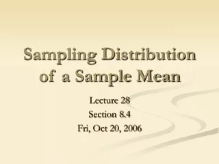
Sampling Distribution of a Sample Mean
Sampling Distribution of a Sample Mean. Lecture 28 Section 8.4 Fri, Oct 28, 2005. Sampling Distribution of the Sample Mean. Sampling Distribution of the Sample Mean – The distribution of sample means over all possible samples of the size n from that population. With or Without Replacement?.

Sampling Distribution of a Sample Mean
E N D
Presentation Transcript
Sampling Distribution of a Sample Mean Lecture 28 Section 8.4 Fri, Oct 28, 2005
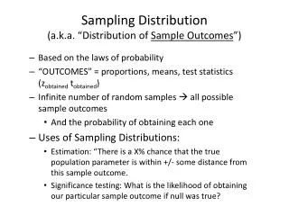
Sampling Distribution of the Sample Mean • Sampling Distribution of the Sample Mean– The distribution of sample means over all possible samples of the size n from that population.
With or Without Replacement? • If the sample size is small in relation to the population size (< 5%), then it does not matter whether we sample with or without replacement. • The calculations are simpler if we sample with replacement. • In any case, we are not going to worry about it.
Example • Suppose a population consists of the numbers {1, 2, 3}. • If we select samples of size n = 3, find the sampling distribution ofx. • Draw a tree diagram showing all possibilities.
The Tree Diagram 1 1 1 2 4/3 3 5/3 1 4/3 2 1 2 5/3 3 2 1 5/3 2 2 3 7/3 3 1 4/3 1 2 5/3 3 2 1 5/3 2 2 2 2 3 7/3 1 2 3 2 7/3 3 8/3 1 5/3 1 2 2 3 7/3 3 1 2 2 2 7/3 3 8/3 1 7/3 3 2 8/3 3 3
The Sampling Distribution • Of the 27 possible samples (equally likely), we find that • 1 sample has an average of 1. • 3 samples have an average of 4/3 = 1.333. • 6 samples have an average of 5/3 = 1.667. • 7 samples have an average of 2. • 6 samples have an average of 7/3 = 2.333. • 3 samples have an average of 8/3 = 2.667. • 1 sample has an average of 3.
The Sampling Distribution • The sampling distribution ofx is
Probability Histogram 7/27 6/27 5/27 4/27 3/27 2/27 1/27 1 2 3
Probability Histogram 7/27 6/27 5/27 4/27 3/27 2/27 1/27 1 2 3
Experiment • We may simulate this on the TI-83 using the function randInt. • The expression randInt(1, 3, 3) will select 3 random numbers from the set {1, 2, 3}, with replacement, and put them in a list.
Experiment • For example, randInt(1, 3, 3) gives {3, 3, 2} which has a sample mean of 2.667. • Generate a list of 100 such sample means, each from a sample of size 3.
Experiment 50 40 30 20 10 1 2 3
Fit a Normal Curve 50 40 30 20 10 1 2 3
Observations • The distribution appears to be centered at . • The distribution appears to be approximately normal (maybe).
Experiment • Now generate a list of 100 sample means, each from a sample of size 30. • Draw the distribution.
Experiment 50 40 30 20 10 1 2 3
Fit a Normal Curve 50 40 30 20 10 1 2 3
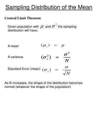
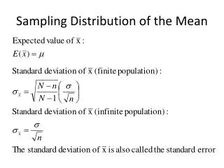
The Central Limit Theorem • Begin with a population that has mean and standard deviation . • For sample size n, the sampling distribution of the sample mean is approximately normal with
The Central Limit Theorem • The approximation gets better and better as the sample size gets larger and larger. • For many populations, the distribution is almost exactly normal when n 10. • For almost all populations, if n 30, then the distribution is almost exactly normal.
The Central Limit Theorem • If the original population is exactly normal, then the sampling distribution of the sample mean is exactly normal for any sample size. • This is all summarized on pages 536 – 537.
Example • Suppose the heights of all adult males has • Mean 68 inches. • Standard deviation 3.6 inches.
Example • The set of sample means from all possible samples of size n = 4 will have • Mean 68 inches. • Standard deviation 3.6/4 = 0.18 inches. • But the distribution will (probably) not be normal.
Example • The set of sample means from all possible samples of size n = 100 will have • Mean 68 inches. • Standard deviation 3.6/100 = 0. 36 inches. • And the distribution will be normal.
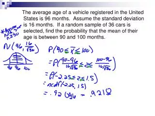
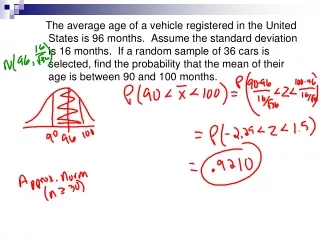
Example • If we collect a sample of 100 adult males from this population, what is the probability that their average height will be at least 67 inches?
Example • The sampling distribution ofx • Is normal (because n 30), • Has mean 68, • Has standard deviation 0. 36. • Therefore, P(x > 67) is given by normalcdf(67, E99, 68, 0.36), which is 0.9973.
Let’s Do It! • Let’s Do It! 8.9, p. 541 – Probability of Accepting the Shipment. • Let’s Do It! 8.10, p. 543 – Mean Grocery Expenditure.
Estimating the Population Mean • Example 8.12, p. 543 – Estimating the Population Mean Grocery Expenditure. • The sampling distribution ofx is approximately normal with • x = $60. • x = $35/100 = $3.50. • Based on the Empirical Rule, 95% of all samples have a mean within $7.00 of $60, that is, between $53 and $67.
Estimating the Population Mean • Suppose that we do not know the true population mean for grocery expenditures, but our sample mean is $58. • What is our best estimate of the true mean? • Point estimate: $58. • Interval estimate: Allow 2 standard deviations either way: $58 $7.