Exploring a Calibrated Solow Model for Argentina: Insights from 1950 SAM Analysis
This paper presents a calibrated Solow model based on a Social Accounting Matrix (SAM) from 1950, focusing on a counterfactual structuralist framework. The model, designed in Excel for transparency, incorporates systematic assumptions including capacity utilization and aggregate demand shocks. Analyzing labor dynamics, it distinguishes between skilled and unskilled labor, accounting for education and experience. Key findings reveal the historical trends and effects of fiscal policy in Argentina, indicating a transition towards government failure and highlighting household decision-making under different economic scenarios.

Exploring a Calibrated Solow Model for Argentina: Insights from 1950 SAM Analysis
E N D
Presentation Transcript
Solow Model • Calibrated to a SAM for 1950 • Usual assumptions • Written in Excel for transparency (instead of GAMS) • Interpretation and changes are straightforward • Produces a counterfactual
Structuralist Model • Calibrated to the same SAM • Uses capacity generated by Solow model
Investment function • u: capacity utilization u = X/Q • X: aggregate demand • Expected rate of profit relative to the cost of capital
Expected profit rate Last period’s profit rate plus a random error term (uniform distribution) rt = rt-1+ ε
Aggregate Demand • X = X(u; ρ*,ρ)+εwhere • ρ∗ foreign savings • ρ govt investment less govt savings • ρ* and ρ are “shocks” (in terms of % of GDP) • Supply determined by Solow model
Labor Market • Supply: exogenous growth rate • Demand: follows productivity and real wages • Walrasian adjustment with lag
The Shocks Two ways to model them • Historical trend (average rate of growth) • Actual data (year by year)
Conclusion • Fiscal policy stabilizing until late 1980s- 1990s. • Se vayan todos: classic government failure ∙ • Argentina and Washington Consensus
Households • 75 households (1950) to 234 households (2000) • Two labor categories: Skilled and unskilled
To enter the skilled labor market • Requires “skill” obtained through • Education or previous experience • Luck
Points system • All labor contracts are renegotiated each period • Education one point • Experience Lt = 1+(1/Lt-1) • Recent experience (last period) • Luck (according to a random variable)
Simulation Design • Excess supply of skilled labor • Some skilled labor bias built into the model • A worker without skill can at best equal a worker with skill (never preferred).