The Solow Growth Model

1. The Solow Growth Model

2. Model Background The Solow growth model is the starting point to determine why growth differs across similar countries it builds on the Cobb-Douglas production model by adding a theory of capital accumulation developed in the mid-1950s by Robert Solow of MIT, it is the basis for the Nobel Prize he received in 1987 the accumulation of capital is a possible engine of long-run economic growth

3. Building the Model: goods market supply We begin with a production function and assume constant returns.Y=F(K,L) so… zY=F(zK,zL) By setting z=1/L we create a per worker function.Y/L=F(K/L,1) So, output per worker is a function of capital per worker. We write this as,y=f(k)

4. Building the Model: goods market supply y y=f(k) k • The slope of this function is the marginal product of capital per worker.MPK = f(k+1)–f(k) • It tells us the change in output per worker that results when we increase the capital per worker by one. Change in y Change in k

5. Building the Model:goods market demand We begin with per worker consumption and investment. (Government purchases and net exports are not included in the Solow model). This gives us the following per worker national income accounting identity.y = c+I Given a savings rate (s) and a consumption rate (1–s) we can generate a consumption function.c = (1–s)y …which makes our identity,y = (1–s)y + I …rearranging,i = s*y …so investment per worker equals savings per worker.

6. Steady State Equilibrium The Solow model long run equilibrium occurs at the point where both (y) and (k) are constant. These are the endogenous variables in the model. The exogenous variable is (s).

7. Steady State Equilibrium By substituting f(k) for (y), the investment per worker function (i = s*y) becomes a function of capital per worker (i = s*f(k)). To augment the model we define a depreciation rate (d). To see the impact of investment and depreciation on capital we develop the following (change in capital) formula,dk = i – dk …substituting for (i) gives us,dk = s*f(k) – dk

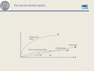
8. The Solow Diagram graphs the production function and the capital accumulation relation together, with Kt on the x-axis: Investment, Depreciation At this point, dKt = sYt, so Capital, Kt

9. The Solow Diagram:When investment is greater than depreciation, the capital stock increases The capital stock rises until investment equals depreciation: At this steady state point, dK = 0 Depreciation: d K Investment: s Y Investment, depreciation Net investment K0 K* Capital, K

10. Suppose the economy starts at K0: Investment, Depreciation K0 K1 Capital, Kt • The red line is above the green at K0: • Saving = investment is greater than depreciation at K0 • So ∆Kt > 0 because • Since ∆Kt >0, Kt increases from K0 to K1 > K0

11. Now imagine if we start at a K0 here: Investment, Depreciation K0 K1 Capital, Kt • At K0, the green line is above the red line • Saving = investment is now less thandepreciation • So ∆Kt < 0 because • Then since ∆Kt<0,Ktdecreases from K0 to K1 < K0

12. We call this the process of transition dynamics: Transitioning from any Kt toward the economy’s steady-state K*, where ∆Kt = 0 and growth ceases Investment, Depreciation No matter where we start, we’ll transition to K*! At this value of K, dKt = sYt, so K* Capital, Kt

13. Changing the exogenous variable - savings Investment, Depreciation dk s*f(k) s*f(k*)=dk* k k* • We know that steady state is at the point where s*f(k)=dk s*f(k*)=dk* s*f(k) • What happens if we increase savings? • This would increase the slope of our investment function and cause the function to shift up. k** • This would lead to a higher steady state level of capital. • Similarly a lower savings rate leads to a lower steady state level of capital.

14. We can see what happens to output, Y, and thus to growth if we rescale the vertical axis: Y* K* Investment, Depreciation, Income • Saving = investment and depreciation now appear here • Now output can be graphed in the space above in the graph • We still have transition dynamics toward K* • So we also have dynamics toward a steady-state level of income, Y* Capital, Kt

15. The Solow Diagram with OutputAt any point, Consumption is the difference between Output and Investment: C = Y – I Investment, depreciation, and output Y0 Y* Investment: s Y Depreciation: d K Consumption K0 K* Capital, K Output: Y

16. Conclusion The Solow Growth model is a dynamic model that allows us to see how our endogenous variables capital per worker and output per worker are affected by the exogenous variable savings. We also see how parameters such as depreciation enter the model, and finally the effects that initial capital allocations have on the time paths toward equilibrium. In the next section we augment this model to include changes in other exogenous variables; population and technological growth.

17. Model Background As mentioned, the Solow growth model allows us a dynamic view of how savings affects the economy over time. We also learned about the steady state level of capital. Now, we assume policy makers can set the savings rate to determine a steady state level of capital that maximizes consumption per worker. This is known as the golden rule level of capital (k*gold)

18. Building the Model: dk* f(k*) • We begin by finding the steady state consumption per worker.From the national income accounts identity, y = c + iwe get c = y – i • We want steady state “c” so we substitute steady state values for both output (f(k*)) and investment which equals depreciation in steady state (dk*) giving us c*=f(k*) –dk* f(k*),dk* • Because, consumption per worker is the difference between output and investment per worker we want to choose k* so that this distance is maximized. • This is the golden rule level of capital k*gold c*gold k* k*gold Above k*gold, increasing k* reduces c* • A condition that characterizes the golden rule level of capital is MPK = d Below k*gold, increasing k* increases c*

19. Building the Model: • While the economy moves toward a steady state it is not necessarily the golden rule steady state. • Any increase or decrease in savings would shift the sf(k) curve and would result in a steady state with a lower level of consumption. f(k*),dk* dk* f(k*) sgoldf(k*) sgoldf(k*) k* k*gold To reach the golden rule steady state… The economy needs the right savings rate.

20. The Transition to the Golden Rule Steady State • Suppose an economy starts with more capital than in the golden rule steady state. • This causes an immediate increase in consumption and an equal decrease in investment. Output, y • Over time, as the capital stock falls, output, consumption, and investment fall. Consumption, c Investment, i • The new steady state has a higher level of consumption than the initial steady state. t0 Time At t0, the savings rate is reduced.

21. The Transition to the Golden Rule Steady State • Suppose an economy starts with less capital than in the golden rule steady state. • This causes an immediate decrease in consumption and an equal increase in investment. Output, y • Over time, as the capital stock grows, output, consumption, and investment increase. Consumption, c Investment, i • The new steady state has a higher level of consumption than the initial steady state. t0 Time At t0, the savings rate is increased.

22. Conclusion In this section we used our knowledge that savings affects the steady state and chose the savings rate to maximize consumption per worker. This is known as the golden rule level of capital (k*gold) In the next section we augment this model to include changes in other exogenous variables; population and technological growth.

23. Model Background As mentioned, the Solow growth model allows us a dynamic view of how savings affects the economy over time. We learned about the steady state level of capital and how a golden rule steady state level of capital can be achieved by setting the savings rate to maximize consumption per worker. We now augment the model to see the effects of population growth and technological progress.

24. Steady State Equilibrium By expanding our model to include population growth our model more closely resembles the sustained economic growth observable in much of the real world. To see how population growth affects the steady state we need to know how it affects the accumulation of capital per worker. When we add population growth (n) to our model the change in capital stock per worker becomes…dk = i – (d+n)k As we can see population growth will have a negative effect on capital stock accumulation. We can think of (d+n)k as break-even investment or the amount of investment necessary to keep capital stock per worker constant. Our analysis proceeds as in the previous presentations. To see the impact of investment, depreciation, and population growth on capital we use the (change in capital) formula from above,dk = i – (d+n)k …substituting for (i) gives us,dk = s*f(k) – (d+n)k

25. Steady State Equilibrium with population growth Break-even investment(d+n)k s*f(k)Investment • At the point where both (k) and (y) are constant it must be the case that,dk = s*f(k) – (d+n)k = 0 …or,s*f(k) = (d+n)k…this occurs at our equilibrium point k*. Like depreciation, population growth is one reason why the capital stock per worker shrinks. InvestmentBreak-even Investment s*f(k*)=(d+n)k* k k* At k* break-even investment equals investment.

26. The impact of population growth • Suppose population growth changes from n1 to n2. • This shifts the line representing population growth and depreciation upward. An increase in “n” InvestmentBreak-even Investment (d+n2)k (d+n1)k • At the new steady state k2* capital per worker and output per worker are lower • The model predicts that economies with higher rates of population growth will have lower levels of capital per worker and lower levels of income. s*f(k) k k2* k1* …reduces k*

27. The efficiency of labour We rewrite our production function as…Y=F(K,L*E)where “E” is the efficiency of labour. “L*E” is a measure of the number of effective workers. The growth of labour efficiency is “g”. Our production function y=f(k) becomes output per effective worker since…y=Y/(L*E) and k=K/(L*E) With this augmentation “dk” is needed to replace depreciating capital, “nk” is needed to provide capital to new workers, and “gk” is needed to provide capital for the new effective workers created by technological progress.

28. Steady State Equilibrium with population growth and technological progress • At the point where both (k) and (y) are constant it must be the case that,dk = s*f(k) – (d+n+g)k = 0 …or,s*f(k) = (d+n)k…this occurs at our equilibrium point k*. Like depreciation and population growth, the labour augmenting technological progress rate causes the capital stock per worker to shrink. Break-even investment(d+n+g)k InvestmentBreak-even Investment s*f(k)Investment s*f(k*)=(d+n)k* At k* break-even investment equals investment. k k*

29. The impact of technological progress • Suppose the worker efficiency growth rate changes from g1 to g2. • This shifts the line representing population growth, depreciation, and worker efficiency growth upward. An increase in “g” InvestmentBreak-even Investment (d+n+g2)k (d+n+g1)k s*f(k) • At the new steady state k2* capital per worker and output per worker are lower. • The model predicts that economies with higher rates of worker efficiency growth will have lower levels of capital per worker and lower levels of income. k k2* k1* …reduces k*

30. Effects of technological progress on the golden rule With technological progress the golden rule level of capital is defined as the steady state that maximizes consumption per effective worker. Following our previous analysis steady state consumption per worker is…c* = f(k*) – (d+ n + g)k* To maximize this…MPK = d+ n + gorMPK – d= n + g That is, at the Golden Rule level of capital, the net marginal product of capital MPK – d, equals the rate of growth of total output, n+g.

31. Steady State Growth Rates in the Solow Model with Technological Progress

32. Conclusion In this section we added changes in two exogenous variables (population and technological growth) to the Solow growth model. We saw that in steady state output per effective worker remains constant, output per worker depends only on technological growth, and that Total output depends on population and technological growth.

33. Strengths and Weaknesses of the Solow Model • The strengths of the Solow model are: • It provides a theory that determines how rich a country is in the long run. • The principle of transition dynamics allows for an understanding of differences in growth rates across countries. • The weaknesses of the Solow model are: • It focuses on investment and capital, while the much more important factor of TFP is still unexplained. • It does not explain why different countries have different investment and productivity rates. • The model does not provide a theory of sustained long-run economic growth.

34. The Model Summarized • Production • The production function: • - has constant returns to scale in capital and labor • - has an exponent of less than 1 (let’s say one-third on capital)  decreasing returns to capital • Variables are time subscripted—they may potentially change over time • Output can be used for either consumption (Ct) or investment (It): Yt = Ct + It • Capital Accumulation • the capital stock next year equals the sum of the capital started with this year plus the amount of investment undertaken this year minus depreciation • Depreciation is the amount of capital that wears out each period ~ 10 percent/year Labor the amount of labor in the economy is given exogenously at a constant level, L Investment the amount of investment in the economy is equal to a constant investment rate, s, times total output, Y It = s Yt Total output is used for either consumption or investment therefore, consumption equals output times the quantity one minus the investment rate Ct = (1 - s) Yt

35. Summary • The starting point for the Solow model is the production model with constant returns to scale in capital and labor with a diminishing marginal product of capital • The capital stock is the sum of past investments. The capital stock today consists of machines and buildings that were bought over the last several decades.

36. The goal of the Solow model is to deepen our understanding of economic growth, but in this it’s only partially successful. The fact that capital runs into diminishing returns means that the model does not lead to sustained economic growth. As the economy accumulates more capital, depreciation rises one-for-one, but output and therefore investment rise less than one-for- one because of the diminishing marginal product of capital. Eventually, the new investment is only just sufficient to offset depreciation, and the capital stock ceases to grow. Output stops growing as well, and the economy settles down to a steady state.

37. There are two major accomplishments of the Solow model. First, it provides a successful theory of the determination of capital, by predicting that the capital-output ratio is equal to the investment-depreciation ratio. Countries with high investment rates should thus have high capital-output ratios, and this prediction holds up well in the data.

38. The second major accomplishment of the Solow model is the principle of transition dynamics, which states that the farther below its steady state an economy is, the faster it will grow. While the model cannot explain long-run growth, the principle of transition dynamics provides a nice theory of differences in growth rates across countries. Increases in the investment rate or total factor productivity can increase a country’s steady-state position and therefore increase growth, at least for a number of years. These changes can be analyzed with the help of the Solow diagram.

39. CHAPTER 5 The Solow Growth Model • In general, most poor countries have low TFP levels and low investment rates, the two key determinants of steady-state incomes. If a country maintained good fundamentals but was poor because it had received a bad shock, we would see it grow rapidly, according to the principle of transition dynamics.