Download
1 / 21
250 likes | 754 Vues
Working with the Solow Growth Model. Mr. Vaughan Income and Employment Theory (402). Lecture Outline. Explaining Stylized Growth Facts “Shock” exogenous variables in SGM and observe results. Assess empirical performance of SGM.

E N D
Working with the Solow Growth Model Mr. Vaughan Income and Employment Theory (402)
Lecture Outline • Explaining Stylized Growth Facts • “Shock” exogenous variables in SGM and observe results. • Assess empirical performance of SGM. • If necessary, “tweak” SGM to improve performance (and re-assess). Total Slides: 21
Solow Growth ModelChange in Savings Rate (s) Analysis Example: Everyone in U.S. raises his savings rate because of experience with credit rationing (2008-09 credit crunch). In short run, increase in saving rate raises growth rate of capital per worker and GDP per capita. Growth rates high during transition to steady state, but decline as k rises. Long-run (steady-state) growth rate of capital per worker and real GDP per worker is zero. In steady state, higher saving rate means higher capital per worker (k2∗>k1∗) and higher GDP per capita, not change in growth rates. Note: Increase in saving rate (s1 to s2) shifts curve more than horizontal line. Δs shifts curve by y/k (APK); Δs shifts horizontal line by δ. Curve shift larger if Y>δK (or Y - δK >0, i.e., NDP exceeds zero). Total Slides: 21
Solow Growth ModelChange in Technology (A) Analysis Example: Advance in finance theory/ computer technology in 1970s. (Note: Discrete advance.) In short run, advance in technology (A) boosts growth rates of capital per worker and GDP per capita. Growth rates remain higher during transition to steady state. In long run, growth rates of capital and real GDP per worker fall to zero. In steady state, higher technology level leads to higher steady-state capital per worker (k2∗> k1∗) and real GDP per capita (y∗), not to changes in growth rates (remains = 0). • Recall: • Production Function: y = A·f(k) • Solow Growth Equation: ∆k/k = s [A·f(k)/k] − sδ− n Total Slides: 21
Solow Growth ModelChange in Population Growth (n)[initial population, and hence, labor input, L(0), constant] Analysis Example: Permanent increase in legal immigration rate. In short run, increase in population growth (n) – other things equal - lowers growth rates of capital per worker and GDP per capita. Growth rates remain lower during transition to steady state. In long run, growth rates of capital and real GDP per worker fall to zero (with/without ∆n). But in steady state, higher population growth leads to lower steady-state capital per worker (k∗> k∗’) and real GDP per capita, not changes in growth rates (= 0). • Recall: • Production Function: y = A·f(k) • Solow Growth Equation: ∆k/k = s [A·f(k)/k] − sδ− n Total Slides: 21
Homework(will not be collected, but could appear in your future) Using Solow Growth Model, analyze impact of: • Increase in labor input (L) • Increase in depreciation (δ) on: • Short-run growth rates of capital per worker & real GDP per capita. • Long-run growth rates of capital per worker & real GDP per capita. • Steady-state levels of capital and real GDP per capita. Note: Answers all in textbook. Total Slides: 21
Solow Growth Model • (+) (+) (−) (−) (0) • k* = k*[ s, A, n, δ, L(0)], where k*[ ] is function mapping variables into k* Total Slides: 21
Convergence • A key question about economic growth is whether poor countries tend to catch up with rich ones (i.e., converge). • i.e., Will sub-Saharan countries catch up with OECD countries? • Approach • What does Solow Growth Model predict about convergence? • How well do stylized facts square with SGM predictions? Total Slides: 21
Solow Growth ModelPredictions about Convergence • Analysis • Economy 1 [poor, k(0)1] starts with lower capital per worker and GDP per capita than Economy 2 [rich, k(0)2]. • Economy 1 grows faster initially because vertical distance between s·(y/k) curve and sδ+nline is greater at k(0)1 than at k(0)2. • Therefore, capital per worker in Economy 1, k1, converges over time toward that in economy 2, k2 (because both are headed for k*) • Prediction: Poor countries will have higher growth rates of capital per worker and GDP per capita than rich countries, other things equal. • Assumptions: • Economies 1, 2 do not trade. • Economies 1, 2, have same production function. • Economies 1, 2 have same k*. Total Slides: 21
Solow Growth ModelPredictions about Convergence • Analysis • NOTE: Same analysis as previous slide. • Economy 1 starts at capital per worker k(0)1 and economy 2 starts at k(0)2, where k(0)2>k(0)1 • The two economies have same steady-state capital per worker, k*, shown by dashed blue line. • In each economy, k rises over time toward k*. However, k grows faster in economy 1 because k(0)1 is less than k(0)2. • Therefore, k1 converges over time toward k2. • Prediction: Poor countries will have higher growth rates of capital per worker and GDP per capita than rich countries, other things equal. • Assumptions: • Economies 1, 2 do not trade. • Economies 1, 2, have same production function. • Economies 1, 2 have same k*. Total Slides: 21
Solow Growth ModelConvergence • SGM model says poor country—with low capital and real GDP per worker—will grow faster than rich one. Logic: • Recall average product of capital (y/k) is diminishing. • Poor country starts with smaller capital stock per worker, so it has higher APK. • SGM predicts poorer countries converge over time to richer ones in terms of capital per worker and real GDP per worker. • Empirical Implication: If countries are plotted on 2 data points – 1960 real GDP per capita and 1960-2000 growth rate – and line is fit to resulting scatterplot, “line of best fit” will have negative slope. Total Slides: 21
Solow Growth Model Evidence on Convergence • Problem • Hypothesis: Relationship between initial GDP per capita and subsequent growth rate should be negative. • Evidence: Not much pattern in data, and what exists appears positive. • PotentialExplanations: • Crummy Theoretical Model • Crummy Empirical Model Total Slides: 21
Solow Growth ModelEvidence on Convergence • Problem • Hypothesis: Relationship between initial GDP per capita and subsequent growth rate should be negative. • Evidence: Not much pattern in crude data, and what exists appears positive. • PotentialExplanations: • Crummy Theoretical Model • Crummy Empirical Model • Looking at OECD only provides homogeneity (i.e., closer to “other things equal”) • Predicted negative relationship emerges. • Note Portugal, Greece, Spain Ireland, in particular. Total Slides: 21
Solow Growth Model Evidence on Convergence • Problem • Hypothesis: Relationship between initial GDP per capita and subsequent growth rate should be negative. • Evidence: Not much pattern in crude data, and what exists appears positive. • PotentialExplanations: • Crummy Theoretical Model • Crummy Empirical Model • Looking at U.S. states provides even more homogeneity (i.e., even closer to “other things equal”). • Predicted negative relationship even stronger. • Not just Civil War states, holds for 4 major regions, too (Northeast, South, Midwest, West). • Holds for different regions in other advanced countries, too. • Note: Figure plots growth of personal income 1880-2000 against level of personal income in 1880 (because gross state product unavailable). Total Slides: 21
Solow Growth Model Evidence on Convergence Upshot: • Similar economies tend to converge. • Dissimilar economies show no relationship betweenlevels and growth rates of real GDP per capita. Explanation? • We assumed determinants of steady-state capital per worker, k*, were the same for all economies. • Reasonable assumption for similar economies, but not for broad range of economies with different economic, political, and social characteristics. Total Slides: 21
Solow Growth Model Allowing for Differences in k*(Example 1) • Analysis • Economy 1 (poor) starts with lower capital per worker than economy 2 (rich): k(0)1 < k(0)2 • Now assume: • Poor economy (1) also has lower saving rate: s1 < s2(reasonable) • But two economies have same technology levels, A, and population growth rates, n. • Implication: Poor economy has lower steady-state capital per power,k*1 < k*2 • Result: Uncertain which economy grows faster initially. • Vertical distance marked with blue arrows could be larger/smaller than one marked with red arrows. • Result: Poor economy (1) does not necessary converge on rich economy (2). Total Slides: 21
Solow Growth Model Allowing for Differences in k*(Example 2) • Analysis • Economy 1 (poor) starts with lower capital per worker than economy 2 (rich): k(0)1 < k(0)2 • Now assume: • Poor economy (1) has higher population growth rate: n1 > n2(reasonable). • Two economies have same technology levels, A, and savings rates, s. • Implication: Poor economy has lower steady-state capital per power, k*1 < k*2 • Result: Uncertain which economy grows faster initially. • Vertical distance marked with blue arrows could be larger/smaller than one marked with red arrows. • Result: Poor economy (1) does not necessarily converge on rich economy (2). Total Slides: 21
Solow Growth Model Implication of Differences in k* • Analysis • NOTE: Same analysis as previous two slides. • Poor economy (1) has lower initial capital per worker than rich economy (2) • [k(0)1<k(0)2] • and also lower steady-state capital per worker. • [k*1 (dashed brown line) < k*2 (dashed blue line)] • Capital per worker converges over time to steady-state value in each country: • Poor economy: k1 (red curve) to k*1 , • Rich economy: k2(green curve) to k*2 . • Result: Since k*1 < k*2 , k1 does not converge to k2 (i.e., poorer country does not have higher growth rate). Total Slides: 21
Solow Growth Model Key Findings on Conditional Convergence ∆k/k = ϕ[k(0), k*] (4.9) (−) (+) In words: Growth rate of capital per worker (and hence real GDP per capita) depends on initial and steady rate levels of capital per worker. Conditional: Relationship holds, if other variable is held constant. Examples: • Holding steady-state capital per worker (k*) constant, higher initial values of capital per worker [k(0)] imply lower growth rates (i.e., getting to nearer steady state requires lower growth rate) • Holding initial capital per worker [k(0)] constant, higher values of steady-state capital per worker (k*) imply higher growth rates (i.e., getting to more distant steady state requires higher growth rate). Total Slides: 21
Solow Growth ModelWhat’s Next? Thus far, model can explain: • Cross-country differences in steady-state living standards (real GDP per capita) • Cross-country differences in capital per worker. • Cross-country differences in growth rates (for similar countries) • Poor countries have higher growth rates of capital per worker and real GDP per capita because of convergence (lower k(0) than rich countries but same k*) • Cross-country differences in growth rates (for dissimilar countries) • Lack of convergence because k*’s differ. We have yet to explain why OECD countries can grow ≈ 2% per year for 100+ years (because SGM says long-run growth rate of real GDP per capita = 0%). Total Slides: 21
Questions over Working with the Solow Growth Model? Mr. Vaughan Income and Employment Theory (402)