The Solow Model
The Solow Model. When 1 st introduced, it was treated as more than a good attempt to have a model that allowed the K/Y= θ to vary as thus avoid the linear relationship between saving and economic growth in the Harrod-Domar Model.

The Solow Model
E N D
Presentation Transcript
The Solow Model • When 1st introduced, it was treated as more than a good attempt to have a model that allowed the K/Y=θ to vary as thus avoid the linear relationship between saving and economic growth in the Harrod-Domar Model. • In its original form, it concludes that the rate of saving (σ) and investment (i) have absolutely no long-run effect on the long-run rate of economic growth. But it allows for economies to transition from short-run, medium-run economic and eventually long-run economic if there is technological progress. • The Solow model has a production function that allows both L & K to be continuously substituted for each other – thus MPK & MPL vary. • Each factor is subject to diminishing returns. Thus, with diminishing returns, continuous investment could not, by itself generate permanent economic growth because diminishing returns would eventually cause the gains from investment to approach zero. • According to Solow, permanent economic growth can only come from technological progress, that is, delaying the onset of diminishing returns. • That said, Solow’s model does not explain how technological progress is achieved. It was left to Schumpeter to explain why firms engage in technological progress.
The Solow Model in Brief • Production Function: Y=F(K,L) with constant returns to scale: cY=F(cK,cL) where c>0. Let c=1/L so that Y/L=F(K/L,1) or • y =f(k) –output per worker. • Convenient since we define economic growth as the change in per capita output. f(k) is subject to diminishing returns. Also y always increases with increase in k. • Consumption and Saving • i=σy where σ is the saving rate. • Stock of capital: • Δk= i – δk = σy - δk = σf(k) - δk • If σf(k) > δk , the capital-labor ratio k will increase and hence will investment. • If σf(k) < δk, that is, depreciation (δ) is so large and diminishing returns have so reduced the marginal gains in output from investment in new capital --- k decreases and so does investment • If σf(k) = δk, then euiulinrium is y* and k*. This is termed the steady state equilibrium --- a terms that defines a situation where all variables grow at the same rate, that is, the growth rates of k and y are zero. • Steady State • Define: gk= Δk/k = [σf(k) /k] – δ • The growth rate of k is positive below k* and negative above k*
The Solow Equilibrium y f(k) y* b δk Linear depreciation σf(k) a Saving function k k*
The Effect of Saving (σ)on the Solow Equilibrium y f(k) y2* y1* δk σ2f(k) a σ1f(k) k k2* k1* With the rate of saving at σ1, the economy’s long-run equilibrium is per-worker capital stock (k1*) and per-worker output is y1* With an increase in the rate of saving (from σ1 to σ2), establishes a new equilibrium at (k2*, y2*) Conclusion: With increases in the rate of saving, the steady state levels of capital per-worker and output per-worker do depend on the rate of saving and investment.
Total factor productivity is defined as the residual between the average growth rate of the factors of production and the growth rate of real output. • 2. According to data, total factor productivity in all 4 Asian Tigers (HK, S. Korea, Singapore, and Taiwan) was zero in Singapore, but comparable to developed economies for the other three. • 3. According to Krugman, the rapid growth rates of Asian Tigers are the result of a transition to a higher steady state equilibrium brought about by sharp increases in saving and the effective labor force. • 4. The Solow model predicts conditional convergence, not absolute convergence, because convergence is conditional on rates of saving, rates of depreciation, rates of technological progress and rates of population growth. The Growth Path with an increase in Saving: Medium but no Permanent Growth y y2* “transitional” medium growth path y1* time t=1 • Suppose the rate of saving increases at t=1. Steady state per worker income increases from y1* to y2* but actual income increases gradually as increased investment increases capital per-worker (k) to its steady-state level. • Note that the increase in per-worker income is largest right after the increase in saving for 3 reasons.
At the beginning of the transition, depreciation (δ) is relatively small because capital stock has not grown much larger • The marginal product of capital (MPK) is still large compared it will be when capital (k) becomes larger. Note: Δk=σf(k) – δk or the size of the change in k each period depends on the difference between the saving curve (σf(k) ) and the depreciation line (δk ). • What the Solow Model has revealed so far. It predicts that: • The economy moves toward a steady-state equilibrium – which is a stable equilibrium. • There is no growth in output or capital stock when the economy reaches its steady state. • When the economy moves from one steady state to another, medium-term growth in per capita output and the per capita capital stock occurs. • The transition from one steady state to another generates only medium-term growth, not permanent growth. • The Solow model does not explain the rate of population growth. However, it does support a lower population growth since a lower n implies a high steady state. This seems to support China’s one-child policy!
The Steady State with Population Growth k f(k) y1* y2* (δ+n)k δk σ1f(k) k k2* k1*
Technological Progress and Permanent Economic Growth Technological progress improves labor efficiency (labor-augmenting technology-technical progress): Y =F[K(L*E) where E is the efficiency of each worker. Thus, we can write our variables in terms of effective labor- product of L and E (L*E) with 1. K/(L*E) will grow only if the capital stock grows more rapidly than the labor force and the level of technology. But because the capital stock is always subject to depreciation, the capital stock per effective worker can only grow if investment per worker ( ) is greater than the sum of (1) the amount that depreciates, (2) the amount of new capital needed to equip additional workers in the labor force, and (3) the amount of capital needed to match technological progress’s effect on the labor’s ability to produce. Note: (1) and (2) imply that investment must cover depreciation ,(δ), and increase the capital stock as fast as the rate of growth of the labor force, which grows at the rate of n. 2. (3) tells us that can remain constant only if capital stock also grows fast enough to cover the growth of effective labor, which grows at rate z – the rate of improvement in labor-augmenting technology. The MPK increases because capital, in effect, has more labor to work with, and thus K and Y can grow at the rate = z + n, without experiencing diminishing returns. Thus capital stock per effective worker changes according to
1.The steady state equilibrium below shows n>0 and z>0. Note that yhat and khat are constant but y =Y/L and k=K/L are constantly growing at the rate of technological progress, z. 2. If is constant, Y must be growing at exactly the rate L*E. If indeed the growth rate of E or z is positive, then Y must be growing faster than L. This means that at steady state, y =Y/L is also growing. Thus, the Solow model now generates economic growth in steady state but it took a positive value for labor-augmenting technological progress to do so. f(k-hat) y-hat (δ+n+z)k-hat y*-hat σ1f(k-hat) k-hat k*-hat The Steady State with Technological Progress
y f3(k) y3 f2(k) f1(k) y2 (δ +n)k y1 σf3(k) σf2(k) σf1(k) k 0 k2 k3 k1 Technological Progress and Economic growth Note: Technological Progress is represented by an upward shift in the production function, f(k)
y The Effect of Technological Progress on Growth –Growth Path y y3 y2 y1 time t=1 t=2 t=3 • Summary • With population growth & technological progress, an economy will transition toward a steady state at a higher level of per capita income output if: • An increase in saving (↑σ); (b) a decrease in its rate of population growth (↓n) • 2. More important, an economy will experience higher continuous economic growth if there is a permanent increase in its rate of labor-enhancing technological progress. • So far: The Solow model explains how medium-run & long-run economic growth is related to saving (σ), population growth (n), and technological progress (z). BUT, these variables are exogenous, i.e. does not explain what determines them or how economic policy might influence them! However, the model does point the direction in examining determinants of long-run economic growth