The Solow Growth Model (Part Two)

1. The Solow Growth Model (Part Two) The golden rule level of capital, maximizing consumption per worker.

2. Model Background • As mentioned in part I, the Solow growth model allows us a dynamic view of how savings affects the economy over time. We also learned about the steady state level of capital. • Now, we assume policy makers can set the savings rate to determine a steady state level of capital that maximizes consumption per worker. This is known as the golden rule level of capital (k*gold)

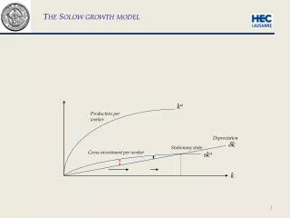
3. Building the Model: δk* f(k*) • We begin by finding the steady state consumption per worker.From the national income accounts identity,y = c + iwe getc = y – i • We want steady state “c” so we substitute steady state values for both output (f(k*)) and investment which equals depreciation in steady state (δk*) giving usc*=f(k*) –δk* f(k*),δk* • Because, consumption per worker is the difference between output and investment per worker we want to choose k* so that this distance is maximized. • This is the golden rule level of capital k*gold c*gold k* k*gold Above k*gold, increasing k* reduces c* • A condition that characterizes the golden rule level of capital isMPK = δ Below k*gold, increasing k* increases c*

4. Building the Model: • While the economy moves toward a steady state it is not necessarily the golden rule steady state. • Any increase or decrease in savings would shift the sf(k) curve and would result in a steady state with a lower level of consumption. f(k*),δk* δk* f(k*) sgoldf(k*) sgoldf(k*) k* k*gold To reach the golden rule steady state… The economy needs the right savings rate.

5. A Numerical Example • Starting with the Cobb-Douglas production function from part I,(1) y=k1/2recall that the following condition holds in steady state,(2) s/δ = k*/f(k*) • assume depreciation is 10% and the policy maker chooses the savings rate and thus the economy’s steady state. Equation (2) becomes,s/.1 = k*/√k*Squaring both sides yields,k* = 100s2 • With this we can compute steady state capital for any savings rate.

6. A Numerical Example • Using the functions from the previous slide and solving for a range of savings rates … • We can see that at s=.5 we get c*=2.5 so at savings rate of .5 consumption per worker is maximized. Also note that at that level MPK–δ=0 and k*=25.

7. A Numerical Example • Another way to identify the golden rule steady state is to choose the level of capital stock where MPK – δ = 0 • In this example MPK = 1/(2√k) – .1 = 0so… 1 = .1(2√k) and… 5 = √kand… 25 = k*

8. A Numerical Example • But what is the time path toward k*? To get this use the following algorithm for each period. • k = 4,andy = k1/2so, y = 2. • c = (1 – s)y, ands = .5soc = .5y = 1.0 • i = s*y, soi = 1.0 • δk = .1*4 = .4 • Δk = s*y – δksoΔk = 1.0 – .4 = .6 • sok = 4+.6 = 4.6for the next period.

9. A Numerical Example • Repeating the process gives… And we converge to k=25

10. The Transition to the Golden Rule Steady State • Suppose an economy starts with more capital than in the golden rule steady state. • This causes an immediate increase in consumption and an equal decrease in investment. Output, y • Over time, as the capital stock falls, output, consumption, and investment fall. Consumption, c Investment, i • The new steady state has a higher level of consumption than the initial steady state. t0 Time At t0, the savings rate is reduced.

11. The Transition to the Golden Rule Steady State • Suppose an economy starts with less capital than in the golden rule steady state. • This causes an immediate decrease in consumption and an equal increase in investment. Output, y • Over time, as the capital stock grows, output, consumption, and investment increase. Consumption, c Investment, i • The new steady state has a higher level of consumption than the initial steady state. t0 Time At t0, the savings rate is increased.

12. Conclusion • In this section we used our knowledge that savings affects the steady state and chose the savings rate to maximize consumption per worker. This is known as the golden rule level of capital (k*gold) • In the next section we augment this model to include changes in other exogenous variables; population and technological growth.