TECHNOLOGICAL PROGRESS AND GROWTH: THE GENERAL SOLOW MODEL
190 likes | 248 Vues
Explore the General Solow Model's insights on economic growth through technological advancements. Learn about steady states, balanced growth rates, and structural policies for prosperity in a closed economy. Dive into the analysis of convergence towards constant levels for capital and labor. Understand the implications of exogenous technological progress on GDP growth per worker.

TECHNOLOGICAL PROGRESS AND GROWTH: THE GENERAL SOLOW MODEL
E N D
Presentation Transcript
Chapter 5 – first lecture Introducing Advanced Macroeconomics: Growth and business cycles TECHNOLOGICAL PROGRESS AND GROWTH: THE GENERAL SOLOW MODEL
The general Solow model • Back to a closed economy. • In the basic Solow model: no growth in GDP per worker in steady state. This contradicts the empirics for the Western world (stylized fact #5). In the general Solow model: • Total factor productivity, , is assumed to grow at a constant, exogenous rate (the only change). This implies a steady state with balanced growth and a constant, positive growth rate of GDP per worker. • The source of long run growth in GDP per worker in this model is exogenous technological growth. Not deep, but: • it’s not trivial that the result is balanced growth in steady state, • reassuring for applications that the model is in accordance with a fundamental empirical regularity. • Our focus is still: what creates economic progress and prosperity…
The micro world of the Solow model … is the same as in the basic Solow model, e.g.: • The same object (a closed economy). • The same goods and markets. Once again, markets are competitive with real prices of 1, and , respectively. There is one type of output (one sector model). • The same agents: consumers and firms (and government), essentially with the same behaviour, specifically: one representative profit maximising firm decides and given and . • One difference: the production function. There is a possibility of technological progress: The full sequence is exogenous and for all . Special case is (basic Solow model).
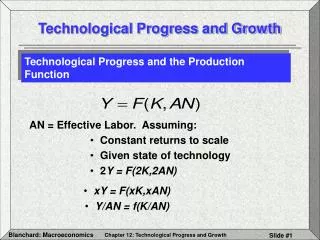
The production function with technological progress with a given sequence, with a given sequence, • With a Cobb-Douglas production function it makes no difference whether we describe technical progress by a sequence, , for TFP or by the corresponding sequence, , for labour augmenting productivity. • In our case the latter is the most convenient. The exogenous sequence, , is given by: • Technical progress comes as ”manna from heaven” (it requires no input of production).
Remember the definitions: and . • Dividing by on both sides of gives the per capita production function: • From this follows: Growth in can come from exactly two sources, and is the weighted average of and with weights and . • If, as in balanced growth, is constant, then !
The complete Solow model • Parameters: . Let . • State variables: and . • Full model? Yes, given and the model determines the full sequences
Note: That is: capital’s share , labour’s share , pure profits . Our should still be around . • Also note: defining ”effective labour input” as :The model is matematically equivalent to the basic Solow model with taking the place of , and taking the place of , and with !We could, in principle, take over the full analysis from the basic Solow model, but we will nevertheless be…
Analyzing the general Solow model • If the model implies convergence to a steady state with balanced growth, then in steady state and must grow at the same constant rate (recall again that is constant under balanced growth). Remember also: Hence if , then . If there is convergence towards a steady state with balanced growth, then in this steady state and will both grow at the same rate as and hence and will be constant. • Furthermore: from the above mentioned equivalence to the basic Solow model, and converge towards constant steady state values. • Each of the above observations suggests analyzing the model in terms of:
and • From we get • From and we get • Dividing by on both sides gives • Inserting gives the transition equation: • Subtracting from both sides gives the Solow equation:
Convergence to steady state:the transition diagram • The transition equation is: • It is everywhere increasing and passes through (0,0). • The slope of the transition curve at any is: • We observe: . Furthermore, . We assume that the latter very plausible stability condition is fulfilled.
Convergence of to the intersection point follows from the diagram. Correspondingly: . Some first conclusions are: • In the long run, and converge to constant levels, and , respectively. These levels define steady state. • In steady state, and both grow at the same rate as , that is, at the rate and the capital output ratio, , must be constant.
Steady state • The Solow equationtogether with gives: • Using and we get the steady state growth paths:
Since , • It also easily follows from that • There is balanced growth in steady state: and grow at the same constant rate, , and is constant. • There is positive growth in GDP per capita in steady state (provided that ).
Structural policies for steady state • Output per capita and consumption per capita in steady state are: • Golden rule: the , that maximises the entire path, . Again: . • The elasticities of wrt. and are again and , respectively. • Policy implications from steady state are as in the basic Solow model: encourage savings and control population growth. • But we have a new parameter, ( corresponds to ). We want a large , but it is not easy to derive policy conclusions wrt. technology enhancement from our model ( is exogenous).
Empirics for steady state • Assume that all countries are in steady state in 2000! • It’s hard to get good data for , so make the heroic assumption that is the same for all countries in 2000. • Set (plausibly) • If is GDP per worker in 2000 of country , the above equation suggests the following regression equation:with and measured appropriately (here as averages over 1960-2000), and where
High significance! Large R2! Even though we have assumed that is the same in all countries! • But always remember the problem of correlation vs. causality. • Furthermore: the estimated value of is not in accordance with the theoretical (model-predicted) value of . Or: • The conclusion is mixed: the figure on the previous slide is impressive, but the figure’s line is much steeper than the model suggests.