The Solow Growth Model
5. The Solow Growth Model. 5.1 Introduction. In this chapter, we learn: how capital accumulates over time, helping us understand economic growth. the role of the diminishing marginal product of capital in explaining differences in growth rates across countries.

The Solow Growth Model
E N D
Presentation Transcript
5 The Solow Growth Model
5.1 Introduction • In this chapter, we learn: • how capital accumulates over time, helping us understand economic growth. • the role of the diminishing marginal product of capital in explaining differences in growth rates across countries. • the principle of transition dynamics: the farther below its steady state a country is, the faster the country will grow. • the limitations of capital accumulation, and how it leaves a significant part of economic growth unexplained. CHAPTER 5 The Solow Growth Model
it builds on the production model by adding a theory of capital accumulation developed in the mid-1950s by Robert Solow of MIT the basis for the Nobel Prize he received in 1987 TheSolow growth modelis the starting point to determine why growth differs across similar countries CHAPTER 5 The Solow Growth Model
The Solow growth model • capital stock is no longer exogenous • capital stock is “endogenized”: converted from an exogenous to an endogenous variable. • the accumulation of capital as a possible engine of long-run economic growth CHAPTER 5 The Solow Growth Model
5.2 Setting Up the Model Start with the production model from chapter 4 and add an equation describing the accumulation of capital over time. Production • The production function: • is Cobb-Douglas • has constant returns to scale in capital and labor • has an exponent of one-third on capital • Variables are time subscripted as they may potentially change over time CHAPTER 5 The Solow Growth Model
Output can be used for either consumption (Ct) or investment (It) A resource constraint describes how an economy can use its resources Capital Accumulation capital accumulation equation: the capital stock next year equals the sum of the capital started with this year plus the amount of investment undertaken this year minus depreciation CHAPTER 5 The Solow Growth Model
Depreciation is the amount of capital that wears out each period the depreciation rate is viewed as approximately 10 percent Thus the change in the capital stock is investment less depreciation represents the change in the capital stock between today, period t, and next year, period t+1 CHAPTER 5 The Solow Growth Model
Labor the amount of labor in the economy is given exogenously at a constant level Investment the amount of investment in the economy is equal to a constant investment rate times total output remember that total output is used for either consumption or investment therefore, consumption equals output times the quantity one minus the investment rate CHAPTER 5 The Solow Growth Model
The Model Summarized CHAPTER 5 The Solow Growth Model
5.3 Prices and the Real Interest Rate • If we added equations for the wage and rental price, the MPL and the MPK would pin them down, respectively -- omitting them changes nothing. • the real interest rate is the amount a person can earn by saving one unit of output for a year • or equivalently, the amount a person must pay to borrow one unit of output for a year • measured in constant dollars, not in nominal dollars CHAPTER 5 The Solow Growth Model
saving is the difference between income and consumption Saving equals investment: a unit of saving is a unit of investment, which becomes a unit of capital: therefore the return on saving must equal the rental price of capital the real interest rate in an economy is equal to the rental price of capital, which is equal to the marginal product of capital CHAPTER 5 The Solow Growth Model
5.4 Solving the Solow Model • To solve the model, write the endogenous variables as functions of the parameters of the model and graphically show what the solution looks like and solve the model in the long run. • combine the investment allocation equation with the capital accumulation equation • netinvestment is investment minus depreciation • substitute the supply of labor into the production function: (change in capital) (net investment) CHAPTER 5 The Solow Growth Model
We now have reduced our system of five equations and five unknowns to two equations and two unknowns: The key equations of the Solow Model are these: The production function And the capital accumulation equation How do we solve this model? We graph it, separating the two parts of the capital accumulation equation into two graph elements: saving = investment and depreciation CHAPTER 5 The Solow Growth Model
Investment, Depreciation At this point, dKt = sYt, so Capital, Kt The Solow Diagram graphs these two pieces together, with Kt on the x-axis: CHAPTER 5 The Solow Growth Model
Depreciation: d K Investment: s Y Investment, depreciation Net investment K0 K* Capital, K Figure 5.1: The Solow Diagram CHAPTER 5 The Solow Growth Model
Using the Solow Diagram • the amount of investment is greater than the amount of depreciation, the capital stock will increase • the capital stock will rise until investment equals depreciation: this point, the change in capital is equal to 0, and absent any shocks, the capital stock will stay at this value of capital forever • the point where investment equals depreciation is called the steady state CHAPTER 5 The Solow Growth Model
Investment, Depreciation K0 K1 Capital, Kt Suppose the economy starts at this K0: • We see that the red line is above the green at K0: • Saving = investment is greater than depreciation • So ∆Kt > 0 because • Then since ∆Kt >0, Kt increases from K0 to K1 > K0 CHAPTER 5 The Solow Growth Model
Investment, Depreciation K0 K1 Capital, Kt Now imagine if we start at a K0 here: • At K0, the green line is above the red line • Saving = investment is now less thandepreciation • So ∆Kt < 0 because • Then since ∆Kt<0,Ktdecreases from K0 to K1 < K0 CHAPTER 5 The Solow Growth Model
Investment, Depreciation No matter where we start, we’ll transition to K*! At this value of K, dKt = sYt, so K* Capital, Kt We call this the process of transition dynamics: Transitioning from any Kt toward the economy’s steady-state K*, where ∆Kt = 0 CHAPTER 5 The Solow Growth Model
when not in steady state, the economy obeys transition dynamics or in other words, the movement of capital toward a steady state notice that when depreciation is greater than investment, the economy converges to the same steady state as above at the rest point of the economy, all endogenous variables are steady transition dynamics take the economy from its initial level of capital to the steady state CHAPTER 5 The Solow Growth Model
Output and Consumption in the Solow Diagram • using the production function, it is evident that as K moves to its steady state by transition dynamics, output will also move to its corresponding steady state by transition dynamics • note that consumption is the difference between output and investment CHAPTER 5 The Solow Growth Model
Y* K* We can see what happens to output, Y, and thus to growth if we rescale the vertical axis: Investment, Depreciation, Income • Saving = investment and depreciation now appear here • Now output can be graphed in the space above in the graph • We still have transition dynamics toward K* • So we also have dynamics toward a steady-state level of income, Y* Capital, Kt CHAPTER 5 The Solow Growth Model
Investment, depreciation, and output Y0 Y* Investment: s Y Depreciation: d K Consumption K0 K* Capital, K Figure 5.2: The Solow Diagram with Output Output: Y CHAPTER 5 The Solow Growth Model
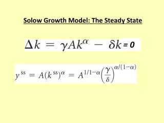
Solving Mathematically for the Steady State • in the steady state, investment equals depreciation. If we evaluate this equation at the steady-state level of capital, we can solve mathematically for it • the steady-state level of capital is positively related with the investment rate, the size of the workforce and the productivity of the economy • the steady-state level of capital is negatively correlated with the depreciation rate CHAPTER 5 The Solow Growth Model
What determines the steady state? • We can solve mathematically for K* and Y* in the steady state, and doing so will help us understand the model better • In the steady state: CHAPTER 5 The Solow Growth Model
If we know K*, then we can find Y* using the production function: CHAPTER 5 The Solow Growth Model
This equation also tells us about income per capita, y, in the steady state: CHAPTER 5 The Solow Growth Model
notice that the exponent on the productivity parameter is greater than in the chapter 4 model: this results because a higher productivity parameter raises output as in the production model. however, higher productivity also implies the economy accumulates additional capital. the level of the capital stock itself depends on productivity CHAPTER 5 The Solow Growth Model
5.5 Looking at Data through the Lens of the Solow Model The Capital-Output Ratio • the capital to output ratio is given by the ratio of the investment rate to the depreciation rate: • while investment rates vary across countries, it is assumed that the depreciation rate is relatively constant CHAPTER 5 The Solow Growth Model
Empirically, countries with higher investment rates have higher capital to output ratios: CHAPTER 5 The Solow Growth Model
Differences in Y/L • the Solow model gives more weight to TFP in explaining per capita output than the production model does • Just like we did before with the simple model of production, we can use this formula to understand why some countries are so much richer • take the ratio of y* for a rich country to y* for a poor country, and assume the depreciation rate is the same across countries: 45 = 18 x 2.5 CHAPTER 5 The Solow Growth Model
Now we find that the factor of 45 that separates rich and poor country’s income per capita is decomposable into: A 103/2 = 18-fold difference in this productivity ratio term A (30/5)1/2 = 61/2 = 2.5-fold difference in this investment rate ratio In the Solow Model, productivity accounts for 18/20 = 90% of differences! 45 = 18 x 2.5 CHAPTER 5 The Solow Growth Model
5.6 Understanding the Steady State • the economy will settle in a steady state because the investment curve has diminishing returns • however, the rate at which production and investment rise is smaller as the capital stock is larger • a constant fraction of the capital stock depreciates every period, which implies depreciation is not diminishing as capital increases CHAPTER 5 The Solow Growth Model
In summary, as capital increases, diminishing returns implies that production and investment increase by less and less, but depreciation increases by the same amount . • Eventually, net investment is zero and the economy rests in steady state. • There are diminishing returns to capital: less Yt per additional Kt • That means new investment is also diminishing: less sYt = It • But depreciation is NOT diminishing; it’s a constant share of Kt CHAPTER 5 The Solow Growth Model
5.7 Economic Growth in the Solow Model • there is no long-run economic growth in the Solow model • in the steady state: output, capital, output per person, and consumption per person are all constant and growth stops both constant CHAPTER 5 The Solow Growth Model
empirically, economies appear to continue to grow over time thus capital accumulation is not the engine of long-run economic growth saving and investment are beneficial in the short-run, but diminishing returns to capital do not sustain long-run growth in other words, after we reach the steady state, there is no long-run growth in Yt (unless Lt or A increases) CHAPTER 5 The Solow Growth Model
5.8 Some Economic Experiments • while the Solow model does not explain long-run economic growth, it does help to explain some differences across countries • economists can experiment with the model by changing parameter values An Increase in the Investment Rate • the investment rate increases permanently for exogenous reasons • the investment curve rotates upward, but the deprecation line remains unchanged CHAPTER 5 The Solow Growth Model
Investment, depreciation New investment exceeds depreciation Depreciation: d K Old investment: s Y K* K** Capital, K Figure 5.4: An Increase in theInvestment Rate CHAPTER 5 The Solow Growth Model
the economy is now below its new steady state and the capital stock and output will increase over time by transition dynamics the long run, steady-state capital and steady-state output are higher What happens to output in response to this increase in the investment rate? the rise in investment leads capital to accumulate over time this higher capital causes output to rise as well output increases from its initial steady-state level Y* to the new steady state Y** CHAPTER 5 The Solow Growth Model
Investment, depreciation, and output New investment: s ‘Y Y** Y* Depreciation: d K Old investment: s Y K* K** Capital, K Figure 5.5: The Behavior of Output Following an Increase in s Output: Y (a) The Solow diagram with output. CHAPTER 5 The Solow Growth Model
Output, Y (ratio scale) Y** Y* 2000 2020 2040 2060 2080 2100 Time, t Figure 5.5:The Behavior of Output Following an Increase in s (cont.) (b) Output over time. CHAPTER 5 The Solow Growth Model
A Rise in the Depreciation Rate • the depreciation rate is exogenously shocked to a higher rate • the depreciation curve rotates upward and the investment curve remains unchanged • the new steady state is located to the left: this means that depreciation exceeds investment • the capital stock declines by transition dynamics until it reaches the new steady state • note that output declines rapidly at first but less rapidly as it converges to the new steady state CHAPTER 5 The Solow Growth Model
Investment, depreciation Old depreciation: d K New depreciation: d ‘K Depreciation exceeds investment Investment: s Y K** K* Capital, K Figure 5.6:A Rise in the Depreciation Rate CHAPTER 5 The Solow Growth Model
What happens to output in response to this increase in the depreciation rate? the decline in capital reduces output output declines rapidly at first, and then gradually settles down at its new, lower steady-state level Y** CHAPTER 5 The Solow Growth Model
Investment, depreciation, and output Investment: s Y Y** Y* New depreciation: d‘K Old depreciation: dK K** K* Capital, K Figure 5.7:The Behavior of Output Following an Increase in d Output: Y (a) The Solow diagram with output. CHAPTER 5 The Solow Growth Model
Output, Y (ratio scale) Y** Y* 2000 2020 2040 2060 2080 2100 Time, t Figure 5.7:The Behavior of Output Following an Increase in d (cont.) (b) Output over time. CHAPTER 5 The Solow Growth Model
Experiments on Your Own • Try experimenting with all the parameters in the model: • Figure out which curve (if either) shifts. • Follow the transition dynamics of the Solow model. • Analyze the steady-state values of capital, output, and output per person. CHAPTER 5 The Solow Growth Model
5.9 The Principle of Transition Dynamics • when the depreciation rate and the investment rate were shocked, output was plotted over time on a ratio scale • ratio scale allows us to see that output changes more rapidly the further we are from the steady state • as the steady state is approached, growth shrinks to zero CHAPTER 5 The Solow Growth Model
the principle of transition dynamics says that the farther below its steady state an economy is, in percentage terms, the faster the economy will grow similarly, the farther above its steady state, in percentage terms, the slower the economy will grow this principle allows us to understand why economies may grow at different rates at the same time CHAPTER 5 The Solow Growth Model
Understanding Differences in Growth Rates • empirically, OECD countries that were relatively poor in 1960 grew quickly while countries that were relatively rich grew slower • if the OECD countries have the same steady state, then the principle of transition dynamics predicts this • looking at the world as whole, on average, rich and poor countries grow at the same rate • two implications: (1) most countries have already reached their steady states; and (2) countries are poor not because of a bad shock, but because they have parameters that yield a lower steady state CHAPTER 5 The Solow Growth Model

