Download
1 / 56
560 likes | 788 Vues
Yehiam Prior. Four Wave Mixing – a Mirror in Time. Weizmann Institute of Science, Rehovot , Israel Suzdal NLO-50(+) September 2011. It took a long time…. And in 1960 the LASER was invented: Soon to be described as a “solution looking for a problem”. Where was I ?.

E N D
Yehiam Prior Four Wave Mixing – a Mirror in Time Weizmann Institute of Science, Rehovot, Israel Suzdal NLO-50(+) September 2011
It took a long time…. And in 1960 the LASER was invented:Soon to be described as a “solution looking for a problem”
Where was I ? 1960 - 7th grade1970 - student in Jerusalem, deciding to continue my studies in the US1971 - Berkeley, looking for a Thesis advisor Options: Shen, Townes, Hahn1977 - post doc position: Nico Bloembergen1979 – Weizmann Institute (ever since)
How does a laser work ? Monochromatic, Directional, Intense, Coherent
Coherent Incoherent
So, what can we do with these Coherent sources?
Spontaneous Raman spectrum of CHCl3 Direct spontaneous Raman spectrum (from the catalogue)
Dk w1 w1 k2 kCARS w2 wAS k1 k1 WRaman 2w1- w2- wAS = 0 Four Wave Mixing (FWM) and Coherent Anti Stokes Raman Scattering (CARS) Conservation of Momentum (phase matching) Energy conservation Dk = 2k1-k2-kAS= 0
FWM Applications included: • Molecular spectroscopy • Rotational and vibrational dynamics • Solid state fast relaxation phenomena • Photon echoes • Combustion diagnostics • Surface diagnostics • Biological applications • Microscopy • Remote sensing • …….
Spectroscopy can be performed either in the frequency domain or in the time domain. • In the frequency domain, we scan the frequency of excitation (absorption), or the frequency of observation (Spontaneous Raman spectroscopy), etc. • Alternatively, we can capture the time response to impulse excitation, and then Fourier Transform this signal to obtain a frequency domain spectrum. • We are always taught that the choice of one or the other is a matter of convenience, instrumentation, efficiency, signal to noise, etc. but that the derived physical information is the same, and therefore the measurements are equivalent.
Time Resolved Four Wave Mixing • A pair of pulses (Pump and Stokes) excites coherent vibrations in the ground state • A third (delayed) pulse probes the state of the system to produce signal • The delay is scanned and dynamics is retrieved
However, practically ALL CARS and Four Wave Mixing experiments were/are performed in the frequency domain. i.e. one is not directly measuring the molecular polarization (wavefunction) which is oscillating at optical frequencies.
Combined Time Frequency Detection of Four Wave Mixing With: Dr. Yuri Paskover (currently in Princeton) Andrey Shalit
Outline • Time Frequency Detection (TFD) : the best of both worlds • Single Shot Degenerate Four Wave Mixing • Tunable Single Shot Degenerate Four Wave Mixing • Multiplex Single Shot Degenerate Four Wave Mixing • TFD simplified analysis • Conclusions
Time Domain vs. Frequency Domain In this TR-FWM the signal is proportional to a (polarization)2 and therefore beats are possible
Time frequency Detection (CHCl3) Open band: Summation over all frequencies (Δ)
F.T Open band:
Limited Band Detection Summation over 500cm-1 window
Open vs. Limited Detection F.T Open band: F.T Limited band:
Spectral Distribution of the Observed Features 104 cm-1 365 cm-1 Observed frequency: 104 cm-1 Observed detuning : 310 cm-1 Observed frequency: 365 cm-1 Observed detuning : 180 cm-1
However, this is a long measurement, it takes approximately 10 minutes, or >> 100 seconds. In what follows I will show you how this same task can be performed much faster. 1015 times faster, or in < 100 femtoseconds !
Also A. Eckbreth, Folded BOXCARS configuration
Ea Eb Ec Time delay Time Resolved Four Wave Mixing Phase matching ~ 50-100 femtosecond pulses ~ 0.1 mJ per pulse
Spatial Crossing of two short pulses:Interaction regions k3 k1 k3 arrives first k1 arrives first 100 fsec = 30 microns 5mm Beam diameter – 5 mm Different regions in the interaction zone correspond to different times delays
Three pulses - Box-CARS geometry Time delays Spatial coordinates
k2 k1 k3 Pump-probe delay z -y +y k1 first k3 first k2 k1 k3 Pump-probe delay Intersection Region: y-z slice
CH2Cl2 Single Pulse CARS Image
CHBr3 Several modes in the range
Geometrical Effects : Phase mismatching x y z Calculated Measured Shalit et al. Opt. Comm. 283, 1917 (2010)
Spectrum of the central frequency (coherence peak) as a function of the Stokes beam deviation
Measured and calculated tuning curve Measured Calculated
For each time delay, a spectrally resolved spectrum was measured.
k2 k1 k3 Pump-probe delay z -y +y k1 first k3 first k2 k1 k3 Pump-probe delay Intersection Region: y-z slice
Intersection Region: y-z slice z -y +y k1 first k3 first
Intersection Region: y-z slice z -y +y Δ
Time Frequency Detection: Single Shot Image Focusing angle : δ = 3 mrad (CH2Br2)
Time Frequency Detection by Single Shot: Fourier Transformed (CH2Br2)