Least-Squares regression line

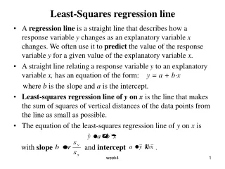
1. Least-Squares regression line • A regression line is a straight line that describes how a response variabley changes as an explanatory variablex changes. We often use it to predict the value of the response variable y for a given value of the explanatory variable x. • A straight line relating a response variable y to an explanatory variable x, has an equation of the form: y = a + b·x where b is the slope and a is the intercept. • Least-squares regression line of y on x is the line that makes the sum of squares of vertical distances of the data points from the line as small as possible. • The equation of the least-squares regression line of y on x is with slope and intercept . week4

2. The slope of the least square regression line, b, is the amount by which y changes when x increase by one unit. • So if the regression line equation is y = a + b·x and we change x to be x+1 (increasing x by 1 unit) the resulting y is y* = a + b·(x + 1) = a + b·x +b. If b > 0 then y will increase and if b < 0, y will decrease. • The change in the response variable y corresponding to a change of k units in the explanatory variable x is equal to k·b. week4

3. Example A grocery store conducted a study to determine the relationship between the amount of money x, spent on advertising and the weekly volume y, of sales. Six different levels of advertising expenditure were tried in a random order for a six-week period. The accompanying data were observed (in units of $100). week4

4. Below is the scatterplot and Minitab output. Variable N Mean StDev ad.cost 6 1.875 0.771 sales 6 18.62 7.31 Correlation of sales and ad.cost = 0.990, P-Value = 0.000 week4

5. MINITAB Commands: Stat > Regression > Regression The regression equation is sales = 1.00 + 9.39 ad. cost Predictor Coef StDev T P Constant 1.004 1.363 0.74 0.502 ad. cost 9.3937 0.6807 13.80 0.000 S = 1.173 R-Sq = 97.9% R-Sq(adj) = 97.4% • The output above gives the prediction equation: sales = 1.00 + 9.39 ad. cost This can be used (after some diagnostic checks) for predicting sales. For example the predicted sales, when the amount spent on advertising is 15, is . week4

6. Extrapolation • Extrapolation is the use of the regression line for prediction outside the rage of values of the explanatory variable x. Such predictions are often not accurate. • For example, predicting the weekly sales, when the amount spent on advertising is 600$, would not be accurate. week4

7. Interpreting the regression line • The slope and intercept of the least-square line depend on the units of measurement-you can not conclude anything from their size. • The least-squares regression line always passes through the point on the graph of y and x. week4

8. Coefficient of determination - r2 • The square of the correlation (r2) is the fraction of the variation in the values of y that is explained by the least-squares regression of y on x. • The use of r2 to describe the success of regression in explaining the response y is very common. • In the above example, r2 = 0.979 = 97.9%, i.e. 97.9% of the variation in sales is explained by the regression of sales on ad. cost. week4

9. Example from Term test, Summer, ’99 • MINITAB analyses of data on math and verbal SAT scores are given below. Correlations (Pearson) Verbal Math Math 0.275 Cell Contents: Correlation 0.000 P-Value GPA 0.322 0.194 0.000 0.006 The regression equation is GPA = 1.11 + 0.00256 Verbal Predictor Coef StDev T P Constant 1.1075 0.3200 3.46 0.001 Verbal 0.0025560 0.0005333 4.79 0.000 S = 0.5507 R-Sq = 10.4% R-Sq(adj) = 9.9 week4

10. Analysis of Variance Source DF SS MS F P Regression 1 6.9682 6.9682 22.98 0.00 Residual Error 198 60.0518 0.3033 Total 199 67.0200 a) Which of the SAT verbal or math is a better predictor of GPA? b) What percent of the variation in GPA is explainable by the verbal scores? c) By the math scores? d) Indicate directly on the scatterplot below what it is that is minimized when we regress GPA on verbal SAT score. Give its actual numerical value for this regression. week4

11. e) In each case below, either make the prediction, or indicate any reservations about making a prediction, or indicate what should be done in order to make a prediction. i) Predict the GPA of someone with a verbal SAT score of 700. ii) Predict the GPA of someone with a verbal SAT score of 250. iii) Predict the verbal score of someone with a GPA of 3.15. week4

12. Residuals • A residual is the difference between an observed value of the response variable and the value predicted by the regression line. That is, residual = observed y – predicted y = . Residuals are also called ‘errors’ and denoted by e . • A negative value of the residual for a particular value of the explanatory variable x, means that the predicted value is overestimating the true value, i.e. • Similarly, when a residual is positive, the predicted value is underestimating the true value of the response, i.e. week4

13. Example • For the example on sales data above, sales = 1.00 + 9.39 ad. cost When x = 1.0, y = 10.2 and then the residual = = 10.2 – 10.39 = - 0.19. • MINITAB commands: Stat > Regression > Regression and click storage and choose Fits and Residuals. The output is given below, week4

14. Row ad. cost sales FITS1 RESI1 1 1.00 10.2 10.3972 -0.19719 2 1.25 11.5 12.7456 -1.24561 3 1.50 16.1 15.0940 1.00596 4 2.00 20.3 19.7909 0.50912 5 2.50 25.6 24.4877 1.11228 6 3.00 28.0 29.1846 -1.18456 week4

15. Residuals and Model Assumptions • The mean of the least-square residuals is always zero. • A model that allows for the possibility that the observations do not lie exactly on a straight line is the model y = a + bx +e where e is a random error. • For inferences about the model, we make the following assumptions on random errors. • Errors are normally distributed with mean 0 and constant variance. • Errors are independent. week4

16. Residual plots • Residual plots help us assess the model assumptions and the fit of a regression line. • Recommended residual plots include: i) Normal probability plot of residuals, and some other plots such as histogram, box-plot etc. Check for normality. If skewed a transformation of the response variable may help. ii) Plot residuals versus predictor or fitted value. Look for curvature suggesting the need for higher order model or transformations, as shown in the following plot week4

17. Also look for trends in dispersion, e.g. an increasing dispersion as the fitted values increase, in which case the assumption of constant variance of the residuals is not valid and a transformation of the response may help, e.g. log or square root. iii) Plot residuals versus time order (if taken in some sequence) and versus any other excluded variable that you think might be relevant. Look for patterns suggesting that this variable has an influence on the relationship among the other variables. week4

18. Outliers and influential observations • An outlier is an observation that lies outside the overall pattern of the other observations. • Points that are outliers in the y direction of a scatterplot have large residuals, but other outliers need not have large residuals. • An observation is influential for a statistical calculation if removing it would markedly change the result of the calculation. • Points that are outliers in the x direction of a scatterplot are often influential for the least square regression line. week4

19. Example - Term test, Summer, ’99 • MINITAB analyses of data on math and verbal SAT scores are given below. The regression equation is GPA = 1.11 + 0.00256 Verbal Predictor Coef StDev T P Constant 1.1075 0.3200 3.46 0.001 Verbal 0.0025560 0.0005333 4.79 0.000 S = 0.5507 R-Sq = 10.4% R-Sq(adj) = 9.9 Unusual Observations Obs Verbal GPA Fit StDev Fit Residual St Resid 15 405 1.9000 2.1427 0.1089 -0.2427 -0.45 X 40 490 1.2000 2.3600 0.0685 -1.1600 -2.12R 89 361 2.4000 2.0302 0.1310 0.3698 0.69 X 108 759 2.8000 3.0475 0.0954 -0.2475 -0.46 X 113 547 1.4000 2.5056 0.0468 -1.1056 -2.01R 121 780 1.3000 3.1012 0.1057 -1.8012 -3.33RX 127 544 1.4000 2.4980 0.0477 -1.0980 -2.00R 131 578 0.3000 2.5849 0.0401 -2.2849 -4.16R 132 430 2.4000 2.2066 0.0965 0.1934 0.36 X 136 760 1.1000 3.0501 0.0959 -1.9501 -3.60RX week4

20. In the scatterplot below, circle the observations possessing the 3 largest residuals. • Circle below all the values that are outliers in the x-direction, and hence potentially the most influential observations. week4

21. Association and causation • In many studies of the relationship between two variables the goal is to establish that changes in the explanatory variable cause changes in response variable. • An association between an explanatory variable x and a response variable y, even if it very strong, is not by itself good evidence that changes in x actually cause changes in y. • Some explanations for an observed association. The dashed double arrow lines show an association. The solid arrows show a cause and effect link. The variable x is explanatory, y is response and z is a lurking variable. week4

22. Lurking Variables • A lurking variable is a variable that is not among the explanatory or response variables in a study and yet may influence interpretation of relationships among those variables. • Lurking variables can make a correlation or regression misleading. • In the sales example above a possible lurking variable is the type of advertising being used e.g. radio, T.V , street promotion etc. week4

23. Confounding • Two variables are confounded when their effects on a response variable cannot be distinguished from each other. • The confounded variable may be either explanatory variables or lurking variables. • Example 2.26 page 176 in IPS. week4

24. Example (Term test May 98) • MINITAB analyses of data (Reading.mtw) on pre1 and post1 scores are given below The regression equation is Post1 = 1.85 + 0.636 Pre1 Predictor Coef StDev T P Constant 1.852 1.185 1.56 0.123 Pre1 0.6358 0.1158 5.49 0.000 S = 2.820 R-Sq = 32.0% R-Sq(adj) = 31.0% Analysis of Variance Source DF SS MS F P Regression 1 239.74 239.74 30.15 0.000 Residual Error 64 508.88 7.95 Total 65 748.62 Unusual Observations Obs Pre1 Post1 Fit StDev Fit Residual StResid 30 8.0 13.000 6.939 0.404 6.061 2.17R week4

25. Does it make sense to use the equation found by MINITAB’s regression procedure for predicting post1 scores from pre1 scores? Also, circle the most unusual value in the data set. Is this an influential observation? • Comment on the distribution of residuals based on the following plots. week4

26. What do you learn from the following plot? week4

27. d) Describe one problem that can be spotted from a plot like the one above, and then draw what the corresponding plot would have to look like, below. e) From the above plots, would you say that ‘group’ is an important lurking variable in our regression of post1 on pre1? Why (not)? Here are some more MINITAB outputs. The regression equation is Pre1 = 5.72 + 0.504 Post1 Predictor Coef StDev T P Constant 5.7203 0.8026 7.13 0.000 Post1 0.50367 0.09173 5.49 0.000 S = 2.510 R-Sq = 32.0% R-Sq(adj) = 31.0% week4

28. Correlations (Pearson) Pre1 Pre2 Post1 Post2 Pre2 0.335 Cell Contents: Correlation 0.006 P-value Post1 0.566 0.345 0.000 0.005 Post2 0.089 0.206 0.064 0.478 0.097 0.607 Post3 -0.037 0.181 0.470 -0.042 0.766 0.146 0.000 0.738 Stem-and-leaf of Post3 N = 66 Leaf Unit = 1.0 2 3 01 7 3 22333 9 3 45 12 3 667 15 3 899 22 4 0001111 30 4 22222333 (7) 4 4455555 29 4 6677 25 4 88888899999999 11 5 001 8 5 333 5 5 4455 1 5 7 week4

29. For each of the following, make a prediction if you can, and if you cannot explain why. (Assume that the variable ‘group’ may be ignored) i) Predict the post1 score of someone with pre1 score = 45. ii) Predict the pre1 score of someone with post1 score = 10. iii) Predict the post1 score of someone with pre1 score = 11. g) If we regressed post3 on pre2, what proportion of the total variation in post3 scores will by explained by the linear relation? • If the std. dev. of post3 is 50% bigger than the std. dev. of pre2, estimate how much of an increase there is in post3 score corresponding to an increase of 1.0 in pre2, on average. i) Is the std. dev. of post 3 scores closer to 0.1, 0.5, 1, 5, 20, 50? week4

30. Cautions about regression and correlation • Correlation measures only linear association, and fitting a straight line makes sense only when the overall pattern of the relationship is linear. Always plot data before calculating. • Extrapolation (using the regression line to predict value far outside the range of the data that we used to fit it) often produces unreliable predictions. • Correlations and least square regressions are not resistant. Always plot the data and look for potentially influential points. • Lurking variables can make a correlation or regression misleading. Plot residuals against time and against other variables that may influence the relationship between x and y. • High correlation does not imply causation. • A correlation based on averages over many individuals is usually higher than the correlation between the same variables based on the data for less individuals. week4

31. Question from Term Test Oct, 2000 • On the plot below, draw in with bars exactly what is minimized (after squaring and summing) should we fit a least-square line to predict W from Z. b) Here is a scatterplot with a positive association between x and y. Explain how you can change this into a negative association without changing x or y values, but by introducing new information about the data. week4

32. Suppose that in a regression study, the observations are taken one per week, over many weeks. What type of diagnostic should you examine? Draw an example of what you would not like to see in this diagnostic plot, if you want to use your simple regression of y on x. Explain briefly what the problem is. week4

33. d) Consider the scatterplot and the possible fitted line below. For the line drawn above draw a rough picture of the following residual plots. i) Residuals vs x. ii) Histogram of residuals. week4

34. Question from Term Test Oct 2000 In a study of car engine exhaust emissions, nitrogen oxide (NOX) and carbon monoxide (CO), in grams per mile were measured for a sample of 46 similar light-duty engines. a) On the graph below circle the two values that likely had the biggest influence on the slope of the l.s. line fitted to all the data. week4

35. If we were to remove the two most influential observations mentioned above, would the slope of the l. s. line increase or decrease? Here are some MINITAB outputs: The regression equation is NOX = 1.83 - 0.0631 CO Predictor Coef StDev T P Constant 1.83087 0.09616 19.04 0.000 CO -0.06309 0.01011 -6.24 0.000 S = 0.3568 R-Sq = 46.9% R-Sq(adj) = 45.7% Analysis of Variance Source DF SS MS F P Regression 1 4.9562 4.9562 38.92 0.000 Residual Error 44 5.6027 0.1273 Total 45 10.5589 Unusual Observations Obs CO NOX Fit StDev Fit Residual St.Resid 22 23.5 0.8600 0.3465 0.1660 0.5135 1.63 X 24 22.9 0.5700 0.3849 0.1602 0.1851 0.58 X 32 4.3 2.9400 1.5602 0.0644 1.3798 3.93 R week4

36. c) What percent of the total variation in NOX is still left unexplained even after taking into account the CO values? d) How much does the NOX emission change when CO decreases by 10 grams? e) Tom predicts a CO of 13.15 if NOX = 1.0 (using the fitted regression equation in the above output). Do you agree? Explain. f) Jim predicts a NOX of 0.06 if CO = 28. Do you agree? Explain. e) The sum of squared deviations of the NOX measurements about their mean is 10.56. The sum of squared deviations of the NOX values from the l.s. line is less than 10.56. The latter is what percent of the former? We continue with the pursuit of a good prediction equation for prediction of NOX measurements. Have a look at the MINITAB outputs and answer the following. week4

37. First we try deleting the 3 most unusual observations. The regression equation is NOX = 1.85 - 0.0724 CO Predictor Coef StDev T P Constant 1.85109 0.08663 21.37 0.000 CO -0.07243 0.01026 -7.06 0.000 S = 0.2809 R-Sq = 54.8% R-Sq(adj) = 53.7% Analysis of Variance Source DF SS MS F P Regression 1 3.9287 3.9287 49.79 0.000 Residual Error 41 3.2352 0.0789 Total 42 7.1639 Unusual Observations Obs CO NOX Fit StDev Fit Residual StResid 22 19.0 0.7800 0.4749 0.1272 0.3051 1.22 X 25 3. 2.2000 1.6012 0.0585 0.5988 2.18R 26 1.9 2.2700 1.7171 0.0708 0.5529 2.03R week4

38. week4

39. i) What improvements, if any, result (ignoring any residual plots for now)? Explain. B) As an alternative to deleting some observations, maybe we should try a transformation. Let’s try a (natural) log transformation of NOX. week4

40. The regression equation is logNOX = 0.656 - 0.0552 CO Predictor Coef StDev T P Constant 0.65565 0.06916 9.48 0.000 CO -0.055232 0.007272 -7.59 0.000 S = 0.2566 R-Sq = 56.7% R-Sq(adj) = 55.7% Analysis of Variance Source DF SS MS F P Regression 1 3.7989 3.7989 57.68 0.000 Residual Error 44 2.8980 0.0659 Total 45 6.6970 Unusual Observations Obs CO logNOX Fit StDev Fit Residual St Resid 16 15.0 -0.6733 -0.1712 0.0635 -0.5022 -2.02R 17 15.1 -0.7133 -0.1800 0.0644 -0.5333 -2.15R 22 23.5 -0.1508 -0.6440 0.1194 0.4931 2.17RX 24 22.9 -0.5621 -0.6103 0.1152 0.0481 0.21 X 32 4.3 1.0784 0.4187 0.0463 0.6597 2.61R week4

41. i) Comparing the scatterplots using NOX and logNOX with no data deleted, what do you conclude? ii) Compare the regressions using logNOX with the regression of NOX on CO but minus the three unusual observations. Which approach works best? (Discuss the residual plots and any other relevant info). week4

42. Question Refer to Exercise-2.73 page 175 IPS. Some useful MINITAB outputs are given below. Coef Stdev t value p Constant -2.5801 2.7277 -0.9459 0.3536 Rural 1.0935 0.0506 21.6120 0.0000 Df SS MS F p Regression 1 9371.099 9371.099 467.0797 0 Error 24 481.516 20.063 State whether the following statements are true of false. I. 95.1% of the variation in city particulate level has been explained by the model. II. An increase of 10g in the rural particulate level is accompanied by an expected increase of 15g in the city particulate level. • The estimated city particulate level when the rural particulate level is 50g is approximately 52g. IV. Correlation between city and rural particulate levels is 0.951. week4

43. Question Examine the following regression minitab output from a study of the relation between freshman year grade point average, denoted "GPA" and verbal Scholastic Aptitude Test score, denoted "VERBAL": The regression equation is GPA = 0.539 + 0.00362 VERBAL Predicto Coef Stdev t-ratio p Constant 0.5386 0.3982 1.35 0.179 VERBAL 0.0036214 0.0006600 5.49 0.000 s = 0.4993 R-sq = 23.5% R-sq(adj)22.7% Analysis of Variance SOURCE DF SS MS F p Regression 1 7.5051 7.5051 30.10 0.000 Error 98 24.4313 0.2493 Total 99 31.9364 week4

44. - - * * * 1.5+ * * * * * - * ** * ** * * 2 resids - ** * * * **** - * ***2 * * * - * * * * * 2 * 2* 0.0+ * * * 2* * * * * * - * 2 2 * - **2** 2 * - 2 3 2** ** * - * *2 * -1.5+ * 2 * * - * ** * - - - * -+---------+---------+---------+---------+---------+------VERBAL 320 400 480 560 640 720 week4

45. State whether the following statements are true or false. I) 23.5% of the variation in GPA's has been explained by the verbal scores. II) An increase of 100 in the verbal SAT score is accompanied by an expected increase of .362 in GPA. III) The estimated GPA for someone attaining a verbal SAT score of 600 is 2.71. IV) Going by the residual plot, we might be better served by using a non-linear model to relate SAT and GPA. V) Since the residual plot shows no pattern, this model will give us very accurate predictions. VI) If the data is normally distributed, the plot above should show a linear pattern. week4