Evolutionary Models and Speciation Patterns Illustrated
Explore various speciation models, from phyletic gradualism to punctuated equilibrium, using phylogenetic diagrams of species diversification over time. This collection showcases evolutionary dynamics and lineage evolution in different organisms and environments.

Evolutionary Models and Speciation Patterns Illustrated
E N D
Presentation Transcript
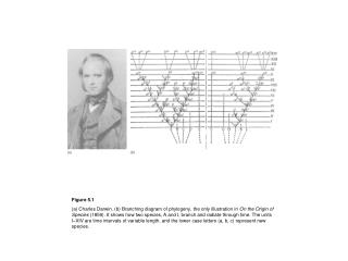
Figure 5.1 (a) Charles Darwin. (b) Branching diagram of phylogeny, the only illustration in On the Origin of Species (1859). It shows how two species, A and I, branch and radiate through time. The units I–XIV are time intervals of variable length, and the lower case letters (a, b, c) represent new species.
Figure 5.2 Allopatric speciation models, occurring either symmetrically (a), where the parent species is divided into two roughly equal halves by a geographic barrier, or asymmetrically (b), where a small peripheral population is isolated by a barrier. In the first case, two new species may arise; in the second, the parent species may continue unaltered, and the peripheral population may evolve rapidly into a new species.
Figure 5.3 Two models of speciation and lineage evolution. (a) Phyletic gradualism, where evolution takes place in the lineages, and speciation is a side effect of that evolution. (b) Punctuated equilibrium, where most evolution is associated with speciation events, and lineages show little evolution (stasis).
Figure 5.4 Fine-scale evolution in fresh-water snails and bivalves in Lake Turkana, Kenya, through the last 4 myr. The volcanic tuff beds allow accurate dating of the sequence. Major speciation events seem to take place at times of lake-level change: are these examples of punctuational speciation, or merely ecophenotypic shifts? (Based on Williamson 1981.)
Figure 5.5 Phyletic gradualism and speciation in the planktonic diatom Rhizosolenia. Today there are two distinct species, R. bergonii and R. praebergonii, that do not interbreed and that differ in the height of the hyaline area. When tracked back through the past 3.4 myr, the species can be seen to have diverged through a span of up to 500,000 years, from 3.2 to 2.7 Ma. The plot shows samples taken from deep-sea boreholes in the central Pacific, and each measurement of the height of the hyaline area is based on a large sample of hundreds of individuals; the means and 95% error bars for each sample are shown. The rock succession is dated by reference to the magnetostratigraphic scheme of normal (black) and reversed (white) polarity. (Courtesy of Ulf Sorhannus.)
Figure 5.6 Punctuated evolution and speciation in the bryozoan Metrarabdotos in the Caribbean. Today, there are three species of this genus, but there have been many more in the past. Careful collecting throughout the Caribbean has shown how the lineages exhibited stasis for long intervals, and then underwent phases of rapid species splitting, especially in the time from 8 to 4 Ma, the Dominican sampling interval (DSI), where records are particularly good. (Courtesy of Alan Cheetham.)
Figure 5.7 Reconstructed phylogeny of African antelopes. Two lineages diverged 6–7 Ma, the slowly evolving impalas and the rapidly speciating gnus and hartebeests. The second group could be said to be evolutionarily more successful than the first, and this might be interpreted as a result of species selection of species-level characters – the rate of speciation. However, the gnus and hartebeests have more specialized ecological preferences than do the species of impalas: perhaps selection has occurred at the individual level (natural selection), and this has had an effect at the species level. Species numbers 14 and 26 are omitted in this study. (Based on Vrba 1984.)
Figure 5.8 Reconstructing the phylogeny of vertebrates by cladistic methods. (a) Are the defining features of vertebrates the possession of bone, a skull and a tail? (b) The tail is found in a wider group, termed the Chordata, but the skull and bone define the Vertebrata.
Figure 5.9 Swimming forepaddles of a variety of reptiles (a–d) and mammals (e–g): (a) Archelon, a Cretaceous marine turtle; (b) Mixosaurus, a Triassic ichthyosaur; (c) Hydrothecrosaurus, a Cretaceous plesiosaur; (d) Plotosaurus, a Cretaceous mosasaur; (e) Dusisiren, a Miocene sea-cow; (f) Allodesmus, a Miocene seal; and (g) Globicephalus, a modern dolphin. The forelimbs are all homologous with each other, and with the wing of a bird and the arm of a human. However, as paddles, these are all analogs: each paddle shown here represents a separate evolution of the forelimb into a swimming structure.
Figure 5.10 The relationships of the major groups of vertebrates, tested using six familiar animals. (a) Postulated relationships, based on the analysis of characters discussed in the text. (b) Phylogenetic tree, showing the cladogram from (a) set against a time scale, and basing the dating of branching points on the oldest known fossil representatives of each group.
Figure 5.11 Relationships of the woolly mammoth based on mitochondrial DNA (mtDNA). This analysis (Rogaev et al. 2006) places the mammoth Mammuthus primigenius closest to the Asiatic elephant Elephas maximus, while other analyses of mammoth mtDNA place the mammoth closer to the African elephant Loxodonta africana. Either way, the relationship to the modern elephants is close, suggesting all three species diverged in the last 5–6 myr. Two samples of mtDNA for the two modern elephants are included, and the outgroups are the sea cow Dugong dugon and the hyrax Procavia capensis. The sets of digits at each branching point are various measures of robustness: values range from 0 to 1 and 0 to 100, with 1.0 and 100% indicating maximum robustness of the node. Scale bar is 0.1 base-pair substitutions per site. (Courtesy of Evgeny Rogaev.)
Figure 5.12 The number of unique trees for three (a) and four (b) taxa. These cladograms may be written more simply as (A(BC), (B(AC)) and ((AB)C) for the three-taxon cases, and ((AB)(CD)), ((AC)(BD)), ((AD)(BC)), etc. for the four-taxon cases. Note that (A(BC)) and (A(CB)) are identical trees, and both versions count as one.