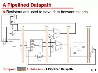
Download

1 / 76
760 likes | 929 Vues
RaPiD The Reconfigurable Pipelined Datapath. Presented and Slides Created by Shannon Koh Based on material from the University of Washington CSE’s RaPiD Project (some images from website, talks and papers). Overview. Motivation Architecture Design Datapath Control Memory

E N D
RaPiDThe ReconfigurablePipelined Datapath Presented and Slides Created by Shannon Koh Based on material from the University of Washington CSE’s RaPiD Project (some images from website, talks and papers)
Overview • Motivation • Architecture Design • Datapath • Control • Memory • Benchmark Architecture • General Architecture • RaPiD-C • Compilation
Motivation • Large data sets and computational requirements; e.g. • Motion Estimation for Real-Time Video Encoding • Accurate Low-Power Filtering for Wireless Comm. • Target architectures include: • General Purpose Processors (including DSPs) • Application-Specific Integrated Circuits (ASICs) • Field-Programmable Compute Engines
Target Arch. Alternatives Fully-Customised Architectures (ASICs) General Purpose Processors Configurable Computing Flexibility Performance • Target applications should have: • More computation than I/O • Fine-grained parallelism • Regular structure
General Purpose Processors • Most flexible architectures • Substantial die area allocated to: • Data and instruction caches • Crossbar interconnect of functional units • Speculative execution and branch prediction • Can extract some instruction-level parallelism • But not large amounts of fine-grained parallelism in compute-intensive applications
ASICs • Higher performance (specific application, entirely inflexible) • Lower cost, BUT: • High non-recurring engineering costs • Speeds up only one application • Only good for applications which are: • Well-defined • Wide-spread
Field-Programmable Computing • Bridging flexibility and performance • Reconfigurable to suit current application needs • BUT, Implemented using FPGAs • Very fine-grained, therefore overhead due to generality is expensive (area and performance) • Programming FPGAs is either: • Poor in density or performance (using synthesis tools) • Requires intimate knowledge of the FPGA (manually)
The Solution? • Given a restricted domain of computations, use reconfiguration to obtain a: • Cost advantage (one chip, many applications) • Performance advantage (customised to the domain) • How? • Many customised functional units (hundreds) • Data cache → Directly streamed to/from external memory • Instruction cache → Configurable controllers • Global register file → Distributed registers/small RAMs • Crossbar interconnect → Segmented buses
Pros and Cons • Pro: Removal of caches, crossbars and register files frees up area that could be used for compute resources • Pro: Communication delay is reduced by shortening wires • Con: Reduces types of applications (e.g. highly irregular, little reuse, little fine-grained parallelism) • Pro: Regular computation-intensive tasks like DSP, scientific, graphics and communications applications will be better over G.P. architectures, and is more flexible than an ASIC.
Overview • Motivation • Architecture Design • Datapath • Control • Memory • Benchmark Architecture • General Architecture • RaPiD-C • Compilation
Datapath Architecture • Hundreds of functional units; broad complexity range • Coarse-grained, word-based • Linearly arranged with word-based buses • Simplifies layout and control • Tightly spaced, no corner turning switches • Multidimensional algorithms can be mapped • Exceptions/control handled by tag bit in data value (propagated to future function units)
Functional Units • Interconnect → Computation → Interconnect • ConfigDelay allows for deeper pipelining • Examples include ALUs, multipliers, shifters, memory, specific functions (e.g. LUTs, no control input), configurable functions (e.g. bit manipulations)
ConfigDelay Unit • Delay by up to three registers • Deeper pipelining
Configurable Interconnect • A set of segmented tracks running the entire length of the datapath • Segmented buses are connected with bus connectors • Left/Right/Both Driving • ConfigDelay included • Double-width data can be output to two tracks and input to two functional units
Cells • Functional units are grouped to form a cell • Cells are replicated to form the entire datapath
0 1 ConfigDelay w w Drive right? Drive left? Bus Connector
Overview • Motivation • Architecture Design • Datapath • Control • Memory • Benchmark Architecture • General Architecture • RaPiD-C • Compilation
Control Architecture • Control bits used in interconnect (multiplexer, tristate drivers, ConfigDelay and bus connectors) and function units • Static field-programmable bits • Too inflexible – only good for static dataflow networks • Programmed control • Too wide, therefore very expensive per cycle
Application Domain (Revisit) • Pipelined computations which are very repetitive • Spend most of the time in deeply nested computation kernels • Soft control is statically compiled • How should we design the control architecture?
FPGA Control FPGA • State machines mapped to an FPGA • Not very efficient due to performance of FPGA • But, easy to reconfigure
Programmed Control Programmed Controller • Dedicated controller • Better performance • Less flexibility • VLIW still expensive (area and performance*)
Reducing Instruction Length • Most of the soft control is constant per application • Regularity of computations allow much of the soft control to control more than one operation in more than one pipeline stage • Reduce controller size • Add a configurable control path
Controller and Decoder Small Programmed Controller Configurable Control Path
Instruction Generator for i = 0 to 9 for j = 0 to 19 for k = 0 to 29 if (k == 0) load reg; if (j <= 3) inc ram addr; if (k > 5) w += w * y; if (k == 0 && j > 3) w = 0; 1xxx x1xx xx1x xxx1
Instruction Tree i = 0 to 9 j = 0 to 3 j = 4 to 19 k = 0 k = 1 to 5 k = 6 to 29 k = 0 k = 1 to 5 k = 6 to 29 1100 0100 0110 1001 0000 0010 for i = 0 to 9 for j = 0 to 19 for k = 0 to 29 if (k == 0) 1xxx; if (j <= 3) x1xx; if (k > 5) xx1x; if (k == 0 && j > 3) xxx1;
Instructions i = 0 to 9 j = 0 to 3 j = 4 to 19 k = 0 k = 1 to 5 k = 6 to 29 k = 0 k = 1 to 5 k = 6 to 29 1100 0100 0110 1001 0000 0010 loop 10 end1 loop 4 end2 inst 1 1100 inst 5 0100 end2: inst 24 0110 loop 16 end1 inst 1 1001 inst 5 0000 end1: inst 24 0010 halt C-Instructions
Instruction Controller loop 10 end1 loop 4 end2 inst 1 1100 inst 5 0100 end2: inst 24 0110 loop 16 end1 inst 1 1001 inst 5 0000 end1: inst 24 0010 halt
Parallel Loop Nests • Single controller – cross product of two loop nests to generate words (not good) • Multiple controllers each executing one loop • Synchronisation using primitives: • signal NUM : indicates that controller number “NUM” should stop waiting or skip to its next wait if not waiting • wait I : repeats instruction word “I” until a signal arrives
Controller S Y N C M E R G E R E P E A T Controller Configurable Control Path Controller Controller Parallel Loop Control • Synchronisation handled by sync unit (signal, wait) • Merge unit may be a bitwise OR or PLA if required • Repeat unit handles repeat instruction repeats (inst)
Overview • Motivation • Architecture Design • Datapath • Control • Memory • Benchmark Architecture • General Architecture • RaPiD-C • Compilation
Memory Architecture • Sequences of memory references are mapped to address generators • Input FIFOs are filled from memory and output FIFOs are emptied to memory
Memory Requirements • Memory interface routes between streams and external memory modules • High bandwidth through: • Fast SRAM • Aggressive interleaving and/or batching • Out-of-order handling of addresses • Sustained data transfer of three words/cycle • May also stream from external sensors
Address Generators • Resembles programmed controller but produces addresses • Addresses packaged with count and stride • Repeaters increment addresses by the stride
Address Generators (Cont’d) • Addressing pattern statically determined at compile time • Timing is determined by control bits • Synchronisation achieved by halting the RaPiD array when: • FIFO is empty on a read • FIFO is full on a write
Overview • Motivation • Architecture Design • Datapath • Control • Memory • Benchmark Architecture • General Architecture • RaPiD-C • Compilation
Benchmark Architecture • Application domain consists primarily of signal-processing applications • Requires high-precision multiply-accumulates • 16-bit fixed-point datapath with 1616 multipliers and 32-bit accumulates • Cell comprises: • 3 ALUs and 3 64-word RAMs • 6 GP Registers and 1 multiplier
Benchmark (Continued) • 14 data tracks • 32 control tracks • 16 replications of the cell • Functional unit mix was chosen based on requirements of a range of signal processing applications
Characteristics • .5μ process (λ = .3μ) • 3.3v CMOS using MOSIS scalable submicron design rules • 100 MHz clock • 16-bit fixed point data, 16 Cells • 16 Multipliers • 48 ALUs • 48 RAMs (64-word) • 14 data buses, 32 control buses
Area Requirements 5.07 mm² for λ = .3μ and 2.25 mm² for λ = .2μ
Configuration Overhead • Straightforward interpretation: triples the area • BUT, hardwired interconnect and control (e.g. FSMs) are called overhead here • Hardwired circuits will not use all functional units or the full data width • Configurable datapath evaluates a variety of computations • Approx. 67% RaPiD but 95-98% for FPGAs
Power Consumption • Optimised for performance rather than power • But, features available for low power applications: • Turn off clocks to unused registers • Tie inputs of unused functional units to ground • Thus, power only used for clocking used units and the clock blackbone
Application Performance • Generally, 1.6 billion MACs per second • FIR Filters • 16 tap, 100 MHz sample rate • 1024 tap, 1.5 MHz sample rate • 16-bit multiply, 32-bit accumulate • Symmetric filter, double performance • IIR Filters • 48 taps at 33.3 MHz