Engineering Systems
Engineering Systems. Shuvra Das University of Detroit Mercy. Summary. Engineering systems Approach to analyze systems System components Types of systems System equations System responses. Flowchart of Mechatronic Systems. Relevant questions: Systems!.

Engineering Systems
E N D
Presentation Transcript
Engineering Systems Shuvra Das University of Detroit Mercy
Summary • Engineering systems • Approach to analyze systems • System components • Types of systems • System equations • System responses
Relevant questions: Systems! • A motor is switched on: “How will the rotation of the shaft vary with time?” • A hydraulic system opens a valve to allow a liquid to flow into a tank: “How will the water level vary with time?” • A crash has occurred: “How fast will the airbag system deploy?” • To answer these questions an understanding of the system behavior is necessary.
Engineering System • A system consists of multiple components that work together to perform a task. Although a system may be made of many components it can be represented as a “black-box” with an input and an output. • temperature measuring system, • transmission system • hydraulic system, • lighting system,heating system • suspension system, etc.
Stages of Dynamic System Investigation • Physical Modeling • Imagine a simple physical model that will match closely the behavior of the system • Equations of Motion • Develop Mathematical Model to describe the physical model • Dynamic Behavior • Study the dynamic behavior of the physical model • Design Decisions • choose physical parameters of the system such that it will behave as desired
ALI KEYHANI MODEL :Mechanical subsystem • The equations for the steering column, pinion and rack can be written : Equation 1 : Equation 2 :
ALI KEYHANI MODEL :Mechanical subsystem Where Td=Torque generated by the driver, Theta1=rotational displacement for the steering column, K2=tire stiffness B2=Viscous damping coefficient B1=friction constant of the upper-steering column X=displacement of the rack m= mass of pinion Ap= Piston area K1=torsion bar stiffness J1=Inertia constant of the upper steering column
ALI KEYHANI MODEL :Mechanical subsystem The following assumptions were made : -the pressure forces on the spool are neglected. -the stiffness of the steering column is infinite. -the inertia of the lower steering column (valve spool and pinion) is lumped into the rack mass.
ALI KEYHANI MODEL hydraulic subsystem By applying the orifice equations to the rotary valve metering orifices and mass conservation equations to the entire hydraulic subsystem the following equation are obtained : Equation 1 : Equation 2 : Equation 3 :
ALI KEYHANI MODEL hydraulic subsystem Where Ps and Po =supply and return pressure of the pump. Pl and Pr = cylinder pressure on the left and right side. Q = supply flow rate of the pump A1 and A2 are the metering orifice area Rho = density of the fluid Beta=bulk modulus of fluid L=length of the cylinder Cd= discharge co-efficient
Neglect small effects Independent environment Lumped characteristics linear relationships constant parameters Neglect uncertainty and noise Realistic physical model leads to non-linear PDEs with time and space varying parameters Simplifying assumptions led to ODEs with constant coefficients Engineering Judgement is key! Examples of approximations
From Physical Model to Mathematical Model • Dynamic Equilibrium Relations: balance of forces, flow rates, energy, etc. which must exist for the system and sub-systems. • Compatibility Relations: how motions of the system elements are interrelated because of the way they are interconnected. • Physical Variables:Selection of precise physical variables (velocity, force, voltage, pressure, flow rate, etc.) with which to describe the instantaneous state of the system.
From Physical Model to Mathematical Model • Physical Laws: Natural Physical laws which individual elements of the system obey, e.g. • Mechanical relations between force and motion • electrical relations between current and voltage • electromechanical relations between force and magnetic field • thermodynamic relations between temperature, pressure, internal energy, etc. • These are also called constitutive physical relationships!
Classification of Physical Variables • Through Variables (one-point variables) measure the transmission of something through an element, e.g. • electric current through a resistor • fluid flow through a duct • force through a spring • heat flux flowing through
Classification of Physical Variables • Across Variables (two-point variables) measures the difference in state between the ends of an element, e.g. • voltage drop across a resistor • pressure drop between the ends of a duct • difference in velocity between the ends of a damper • temperature difference
Equilibrium Relations • Are always relations among through variables • Kirchoff’s current law (at an electrical node) • continuity of fluid flow • equilibrium of forces meeting at a point • heat flux balance
Compatibility Relations • Are always relations among “across variables” • Kirchoff’s voltage law around a circuit • pressure drop across all the connected stages of a fluid system • geometric compatibility in a mechanical system
Physical Relations • Are relations between through and across variables of each individual element, e.g. • f = k.x for a spring • I=V/R for a resistor
spring mass damper capacitor Voltage generator resistor inductor Hydraulic valves ….. A real system, may be broken down into components that behave like one of the basic components System Components
F=force T=torque x=displacement q = angular displacement dx/dt=v=velocity dq/dt=w=angular velocity dv/dt=a=acceleration dw/dt=a=angular acceleration I=inertia m=mass k=spring constant C=damping coefficient Mechanical Quantities
Electrical Quantities • V=voltage • Q=charge • I=current • L=inductance • C=capacitance • R=resistance
F Building Blocks: Mechanical • Translational: • spring; • F = kx (force displacement relationship), • E= 1/2(F2/k), energy stored
F Building Blocks: Mechanical • Translational: • dashpot (damper); • F = C v (C(dx/dt)) (Force-velocity relationship) • E = Cv 2 energy dissipated
F Building Blocks: Mechanical • Translational: • mass; • F = ma = m(d2x/dt2) • E = 1/2 mv2 ,Kinetic Energy
T Building Blocks: Mechanical • Rotational: • Spring; • T = k q, • E = 1/2 (T2/k), energy stored
T Building Blocks: Mechanical • Rotational: • dashpot; • T = C w = C dq/dt • P = Cw2 energy dissipated
T Building Blocks: Mechanical • Rotational: • Moment of Intertia; • T = I d2q/dt2 • E =1/2 I w2 , Kinetic energy
V Building Blocks: Electrical • Capacitor; • Q = CV or V = Q/C, • E = 1/2 CV2 energy stored
V Building Blocks: Electrical • Resistor; • V = IR or V = R (dQ/dt), • energy dissipated E = I2R
V Building Blocks: Electrical • Inductor; • V = L di/dt = L (d2Q/dt2) • E = 1/2 L I2 energy stored
Thermal System • T = Temperature • q = heat flux • R=thermal resistance • Conduction, R=L/Ak, A = cross-sectional area, L=length conducted over, k = thermal conductivity • Convection, R=1/Ah, A = convective surface, h = convective heat transfer coefficient • C=thermal capacitance, mCp (mass X specific heat capacity)
Thermal System • q = (T2-T1)/R • q=Ak(T2-T1)/L; conduction • q=Ah(T2-T1); convection • q1-q2=mCp(dT/dt), q1-q2= rate of change of internal energy
Hydraulic Systems • We will not deal with Hydraulic systems here…...
Types of Systems • Zeroth order systems • First order systems • Second order systems
Example of a First order system • Temperature measuring devices (e.g. thermocouple or a thermometer) are first-order systems. • If a thermometer is dipped in a liquid: • mCp dT/dt = (Ak/L) (TL -T) • where m = mass of bulb, Cp is the specific heat capacity, T is the current temperature of the mercury, A is the surface area of the bulb, k is its thermal conductivity, L is the wall thickness, and TL is the temperature of the liquid.
First order system • Rewritten: • mCp dT/dt + (Ak/L) T = (Ak/L) (TL) • This is a first order system that has been subjected to a step input (which is the right hand side of the above equation) • When this is integrated and initial conditions applied the solution of this system is an exponential function: • T = TL + [T0-TL] e-t/t
First order system • T = TL + [T0-TL] e-t/t • T0 is the temperature of the bulb at intial time; and t, the time constant, is written as (mCpL/Ak). • Response of a First order system to a step input(decaying and progressing)
First order system • Steady state value is TL (target). • How soon is this value reached ? (imp. Question) • The answer lies in the magnitude of the time constant (=mCpL/Ak, in this case). • Time constant is defined as the time required to complete 63.2% of the process, i.e. if the temperature has to rise from 10 degrees to 70 degrees, time constant is the time required to reach (10 +63.2%of the interval) 47.92 degrees.