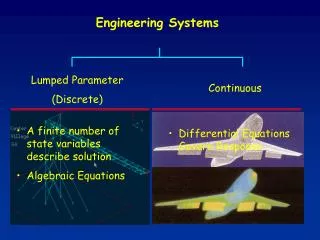
Engineering Systems
This document covers the essentials of lumped parameter systems in engineering mechanics. It discusses the representation of structural displacements through a finite number of state variables, using algebraic and differential equations. The focus is on deriving the stiffness matrix, exploring concepts such as equilibrium, constitutive equations, and compatibility conditions. It emphasizes transformations between local and global coordinate systems, application of boundary conditions, and the properties of the stiffness matrix. Understanding these principles is crucial for effective matrix structural analysis.

Engineering Systems
E N D
Presentation Transcript
Engineering Systems Lumped Parameter (Discrete) Continuous • A finite number of state variables describe solution • Algebraic Equations • Differential Equations Govern Response
Lumped Parameter Displacements of Joints fully describe solution
Matrix Structural Analysis - Objectives Basic Equations Use Equations of Equilibrium Constitutive Equations Compatibility Conditions Form [A]{x}={b} Solve for Unknown Displacements/Forces {x}= [A]-1{b}
Terminology Element: Discrete Structural Member Nodes: Characteristic points that define element D.O.F.: All possible directions of displacements @ a node
Assumptions • Linear Strain-Displacement Relationship • Small Deformations • Equilibrium Pertains to Undeformed Configuration
The Stiffness Method Consider a simple spring structural member Undeformed Configuration Deformed Configuration
Derivation of Stiffness Matrix Using Basic Equations d1 d2 P1 P2
Derivation of Stiffness Matrix Using Basic Equations d2 + d1 = For each case write basic equations
Derivation of Stiffness Matrix Using Basic Equations P21 P11 Equilibrium X d2=0 d1 P11 Constitutive
Derivation of Stiffness Matrix Using Basic Equations P12 P22 Equilibrium d1=0 d2 Constitutive
Derivation of Stiffness Matrix Using Basic Equations P1 P2 Combined Action
Derivation of Stiffness Matrix Using Basic Equations In Matrix Form
Consider 2 Springs 1 2 3 k1 k2 2 elements 3 nodes 3 dof 1 Fix Fix 2 Fix Fix 3 Fix Fix
2-Springs Compare to 1-Spring
Use Superposition d1 d1 d2 d2 0 0 d3 d3 d1 d1 X X X X d2 d2 3 1 2 1 3 2 X X X X d3 d3 DOF not connected directly yield 0 in SM
Properties of Stiffness Matrix • SM is Symmetric • Betti-Maxwell Law • SM is Singular • No Boundary Conditions Applied Yet • Main Diagonal of SM Positive • Necessary for Stability
Apply Boundary Conditions kii kij kik kil kim ui Pi uj Pj kji kjj kjk kjl kjm uk = Pk kki kkj kkk kkl kkm ul Pl kli klj klk kll klm um Pm kli klj klk kll klm -1 uf = Kff (Pf + Kfsus) uf Pf Kff Kfs Ksf Kss us Ps Kffuf+ Kfsus=Pf Ksfuf+ Kssus=Ps Ksfuf+ Kssus=Ps
Transformations Global CS k1 k2 d3 u6 u4 u2 u4 d1 u1 u3 u5 u3 y P x x Local CS d2 d2 Objective: Transform State Variables from LCS to GCS
Transformations P2x P2y Global CS 2 1 f P1x y P1x P1x = P1xcosf + P1ysinf P1y = -P1xsinf + P1ycosf P1y cosf sinf P1x x = P1x -sinf cosf P1y P1y P1 P1 = T Consider
Transformations P2y P2x Global CS 1 2 f P1x or y P1x -1 -1 P1y P2 P1 P1 P2 = = T T Similarly for u x or P2 P1 u1 u2 u2 u1 P1 P2 = = = = T T T T In General
Transformations P1y P2y P2x d1 1 -1 P1 k = 2 1 P2 -1 1 d2 P2 P1x f 1 0 -1 0 u1x P1x 0 0 0 0 u1y P1y P1 = k -1 0 1 0 u2x P2x 0 0 0 0 u2y P2y Element stiffness equations in Local CS Expand to 4 Local dof
SM in Global Coordinate System -1 R K R u P = [T] [0] [R]= K : Element SM in global CS [0] [T] Introduce the transformed variables… Both R and T Depend on Particular Element
Transformations l2 lm - l2 - lm m2 - lm - m2 K = AE/L l2 lm Symm. m2 For example for an axial element with k=AE/L l=cosf m=sinf
In Summary • Derivation of element SM – Basic Equations • Structural SM by Superposition • Application of Boundary Conditions - Elimination • Solution of Stiffness Equations – Partitioning • Local & Global CS • Transformation