Download
1 / 66
680 likes | 928 Vues
Introduction to Neuroimaging. G. Hathout, M.D. Professor, UCLA Dept of Radiology Division of Neuroradiology, West LA VA. Acknowledgements:

E N D
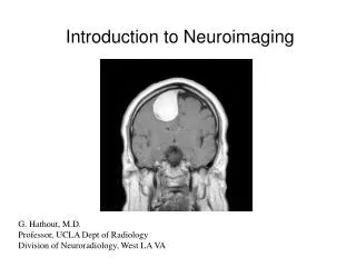
Introduction to Neuroimaging G. Hathout, M.D. Professor, UCLA Dept of Radiology Division of Neuroradiology, West LA VA
Acknowledgements: While most of the slides are mine, I have liberally borrowed slides from the Web to enhance this presentation. I would like to gratefully acknowledge those sources, and to apologize if any have been inadvertently overlooked.
Acknowledgements, cont’d http://www.cs.sunysb.edu/~mueller/teaching/cse377/mriPhysics.pdf http://hsc.uwe.ac.uk/radscience/MRI/MRI_Physics.pdf http://www.mri.tju.edu/phys-web/1-T1_05_files/frame.htm http://www.biac.duke.edu/education/courses/fall03/fmri/handouts/W5_Physics_2003.ppt#256,1,Principles of MRI Physics and Engineering UC San Diego Neuroradiology Learning Files, Dr. Hesselink.
56 y.o. patient, nearly comatose, not moving left side. Diagnosis ?
Neuroradiology: The Old Days!
Introduction to CT (Computer • Assisted Tomography). • Neuroimaging’s first big step: • image in slices • -avoid superposition of structures
CT generates images by taking numerous 2D projections and mathematically reconstructing them to make a planar image.
Rotating X-ray tube and detector array allows multiple projections at different angles. Impact CT scan
The projections can be reconstructed in a number of ways, such as filtered back projection, or using Fourier methods, to form an image.
Each image is made of pixels (picture elements), typically 256 x 256. Each pixel is given a shade of gray, corresponding to its linear attenuation coefficient u. CT (Hounsfield) numbers can be generated from this.
The added information of CT comes at a high price: big radiation doses!
Some actual Hounsfield unit measurements from the scanner – by assigning a CT number to each pixel, CT can make a planar image with good contrast and no overlap! Hounsfield Units White matter: 28 Gray matter: 34 CSF: 4 Fat: -87 Bone: 733
Remember: The higher the electron density, the higher the linear x-ray attenuation coefficient u. The higher u, the higher the CT number (HU or Hounsfiled unit). The higher the HU, the brighter something looks on CT. • Gray matter is about 6 HU higher than white matter (therefore slightly brighter on CT). • Gray matter contains more water and less fat than white matter • This means about 8% more oxygen and 8% less carbon • This leads to a slightly higher electron density (O : 16 vs. C :12) • - This, in turn, leads to higher linear x-ray attenuation
What CT can show: Images can be windowed differently. On “bone” windows, we can distinguish metal from bone. For example, this man decided to stop a bullet with his head. Notice that on bone windows, the brain detail is lost.
Scans show a lentiform hyperdense extra-axial collection pressing on the right cerebral hemisphere (your left, the patient’s right), diagnostic of an epidural hematoma.
There is significant mass effect on the lateral ventricles and midline shift. On bone windows, the hematoma seems to disappear (brain detail is lost), but we can now appreciate the fracture (arrow) which has lacerated the… (fill in the blank).
The patient on your right has blood in the subarachnoid spaces. What is the leading cause of atraumatic subarachnoid bleed?
The ventricles are too big = Hydrocephalus. Notice – the aqueduct of Sylvius is missing (arrow). Diagnosis: Congenital aqueductal stenosis.
Contrast (iodinated compound) can be added to CT. In areas of pathology, it leaks out of a damaged blood-brain barrier. Notice that normal brain does not enhance. Patient has a deep ring-enhancing lesion with surrounding edema, seen only after contrast. Diagnosis: abscess versus tumor (metastatic or primary).
Now, on to the star of neuroimaging: Magnetic Resonance Imaging, a.k.a. MRI MR is a method of mapping hydrogen protons. It not only reflects proton density (like CT reflects electron density), but also reflects magnetic properties of hydrogen protons. This means …. Better tissue contrast!
MRI Imaging in 3 Easy Steps: • Establish equilibrium • Disturb Equilibrium • 3. Allow protons to return to equilibrium
At equilibrium, the multiple hydrogen protons oriented “parallel,” and “anti-parallel,” to the magnetic field produce a state of net vertical magnetization (Mz), but no horizontal magnetization (Mxy = 0). ****Key Point: At equilibrium, there is a net vertical magnetization, but no horizontal magnetization.
The equilibrium is disturbed by radiofrequency pulses which destroy the vertical magnetization Mz and create a horizontal magnetization Mxy. It is this horizontal magnetization Mxy that produces the signal that makes the MR image.
After the RF pulse stops, the system returns to equilibrium.
Important: definition of T1 and T2. T1 and T2 are time constants that measure the speed at which various proton populations return to equilibrium. The T1 time of a tissue reflects how quickly vertical magnetization recovers in that tissue. T1 weighted images reflect the relative T1 times of different tissues. The T2 time reflects how quickly horizontal magnetization disappears in that tissue. T2 weighted images reflect the relative T2 times of different tissues.
Solid tissue has a SHORTER T1 time than free water, so it recovers its longitudinal magnetization faster. Therefore, it has a higher signal than water on T1 weighted images.
For example, pure fat has a shorter T1 time (recovers longitudinal magnetization faster) than white matter, so it is brighter on a T1 weighted image.
Water has a longer T2 time than solid tissue (loses transverse magnetization more slowly), so it is brighter on a T2 weighted image.
Pure water has a longer T2 time than gray matter, so it is brighter (has a higher MR signal) on a T2 weighted image.
Take home message: *On T1 weighted images, tissues with SHORTER T1 times are brighter. *On T2 weighted images, tissues with LONGER T2 times are brighter.
Some representative T1 and T2 times of various tissues (measured in milliseconds)
-Fat has a short T1 time, and water has a long T1 time, so scalp fat is bright and CSF • is dark on a T1 weighted image. • -Water has a long T2 time, so CSF is bright on a T2 weighted image. • -White matter (myelinated) has more fat and less water than gray matter • Therefore, on a T1 weighted image, white matter is brighter than gray matter, • while on a T2 weighted image, white matter is darker than gray matter.
The ability to reflect T1 and T2 times of protons gives much more tissue contrast than just being able to reflect the relative proton density (as in the bland proton density or PD image on the far right, which has very little tissue contrast).
The benefits of contrast resolution! Diagnosis?
Hypoplastic cerebellar vermis leads to an in utero diagnosis of Dandy-Walker malformation!
The benefits of multiplanar imaging Anything missing? (Patient on your left, control on right)
Patient is missing his corpus callosum. Diagnosis: Agenesis of the corpus callosum
T1 weighted MR images of a child – little obvious pathology visible.
After contrast administration, numerous ring enhancing abscesses are visible at the base of the brain. Diagnosis: CNS tuberculosis. Teaching point: Utility of gadolinium contrast in MRI.
42 year old with headache (Slide 1) Ring enhancing lesions in right parietal lobe with edema. Ddx: abscess vs. tumor