Download
1 / 11
110 likes | 188 Vues
Dive into the world of least-squares regression, a vital method for summarizing the relationship between two quantitative variables through a regression line. Explore key concepts, such as residuals, slope, y-intercept, and coefficient of determination to analyze data effectively. Learn about outliers, influential points, and the correlation between slope and correlation. Enhance your data analysis skills with this comprehensive overview of least-squares regression.

E N D
3.3 LEAST-SQUARES REGRESSION (Pages 137 - 160) "The advancement and perfection of mathematics are intimately connected with the prosperity of the state." Napoleon Bonaparte, 1769-1821
Overview: • If a scatterplot shows a linear relationship between two quantitative variables, least-squares regression is a method for finding a line that summarizes the relationship between the two variables, at least within the domain of the explanatory variable, x. • The least-squares regression line (LSRL) is a mathematical model for the data.
Regression Line: • A straight line that describes how a response variable y changes as an explanatory variable x changes. • It can sometimes be used to predict the value of y for a given value of x. • A residual is a difference between an observed y and a predicted y.
Important facts about the least squares regression line. • It is a mathematical model for the data. • It is the line that makes the sum of the squares of the residuals as small as possible. • The point (xbar,ybar) is on the line, where xbar is the mean of the x values, and ybar is the mean of the y values. • Its form is y(hat) = a + bx. (Note that b is slope and a is the y-intercept.)
Important facts continued: • b = r(sy/sx). (On the regression line, a change of one standard deviation in x corresponds to a change of r standard deviations in y.) • a = (ybar) – b(xbar). • The slope b is the approximate change in y when x increases by 1. • The word "approximate" is important here. • The y-intercept a is the predicted value of y when x = 0. • Note that this only has meaning when x can assume values close to 0... and the word "predicted" is important.
r2 in regression: • The coefficient of determination, r2, is the fraction of the variation in the values of y that is explained by the least squares regression of y on x. • Calculation of r2 for a simple example: • r2 = (SSM-SSE)/SSM, where • SSM = sum(y-ybar)2 (Sum of squares about the mean y)SSE = sum(y-y(hat))2 (Sum of squares of residuals)
An example In this example, y(hat) = 2 + 2.25x, the mean of x is 4, and the mean of y is 11. r2 = (SSM-SSE)/SSM = (42-1.5)/42 = 0.9642857143
THINGS TO NOTE: • Sum of deviations from mean = 0. • Sum of residuals = 0. • r2 > 0 does not mean r > 0. • If x and y are negatively associated, then r < 0.
Special Points: • Outlier: • A point that lies outside the overall pattern of the other points in a scatterplot. • It can be an outlier in the x direction, in the y direction, or in both directions. • Influential point: • A point that, if removed, would considerably change the position of the regression line. • Points that are outliers in the x direction are often influential.
Note: • Do not confuse the slope b of the LSRL with the correlation r. • The relation between the two is given by the formula • b = r(sy/sx). • If you are working with normalized data, then b does equal r since sy = sx = 1. • When you normalize a data set, the normalized data has mean = 0 and standard deviation = 1. • If you are working with normalized data, the regression line has the sample form yn = rxn, where xn and yn are normalized x and y values, respectively. • Since the regression line contains the mean of x and the mean of y, and since normalized data has a mean of 0, the regression line for normalized x and y values contains (0,0).
Read Pages 137 to 164 Work 3.31 3.33 3.35 3.36 3.37 3.38 3.39 3.40 For Section 3.3: