Download
1 / 23
240 likes | 581 Vues
3.2 OLS Fitted Values and Residuals. - after obtaining OLS estimates, we can then obtain fitted or predicted values for y:. -given our actual and predicted values for y, as in the simple regression case we can obtain residuals:.

E N D
3.2 OLS Fitted Values and Residuals -after obtaining OLS estimates, we can then obtain fitted or predicted values for y: -given our actual and predicted values for y, as in the simple regression case we can obtain residuals: -a positive uhat indicates underprediction (y>yhat) and a negative uhat indicates overprediction (y<yhat)
3.2 OLS Fitted Values and Residuals -We can extend the single variable case to obtain important properties for fitted values and residuals: 1) The sample average of the residuals is zero, therefore: 2) Sample covariance between each independent variable and the OLS residual is zero… -Therefore the sample covariance between the OLS fitted values and the OLS residual is zero -Since the fitted values come from our independent variables and OLS estimates
3.2 OLS Fitted Values and Residuals Is always on the OLS regression line: 3) The point Notes: These properties come from the FOC’s in (3.13): -the first FOC says that the sum of residuals is zero and proves (1) -the rest of the FOC’s imply zero covariance between the independent variables and uhat (2) -(3) follows from (1)
3.2 “Partialling Out” -In multiple regression analysis, we don’t need formulas to obtain OLS’s estimates of Bj -However, explicit formulas can give us interesting properties -In the 2 independent variable case: -Where rhat are the residuals from regressing x1 on x2 -ie: the regression:
3.2 “Partialling Out” -rhati1 are the part of xi1that are uncorrelated with x12 -rhati1 is equivalent to xi1 after xi2’s effects have been “partialled out” or “netted out” -thus B1hat measures x1’s effect on y after x2 has been “partialled out” -In a regression with k variables, the residuals come from a regression of x1 on ALL other x’s -in this case B1hat measures x1’s effect on y after all other x’s have been “partialled out”
3.2 Comparing Simple and Multiple Regressions -In 2 special cases, OLS will estimate the same B1hat for 1 and 2 independent variables -Write the simple and multiple regressions as: -The relationship between B1hats becomes: -Where delta is the slope coefficient from regressing x1 on x2 (proof in Appendix)
3.2 Comparing Simple and Multiple Regressions -Therefore we have two cases where the B1hats will be equal: 1) The partial effect of x2 on yhat is zero: 2) x1 and x2 are uncorrelated in the sample:
3.2 Comparing Simple and Multiple Regressions -Although these 2 cases are rare, they do highlight the situations where B1hats will be similar -When B2hat is small -There is little correlation between x1 and x2 In the case of K independent variables, B1hat will be equal to the simple regression case if: • OLS coefficients on all other x’s are zero • X1 is uncorrelated with all other x’s -Likewise, small coefficients or little correlation will lead to small differences in B1
3.2 Wedding Example -Assuming decisions in a wedding could be quantified, wedding decisions are regressed on the bride’s opinions to give: -Adding the groom’s opinions gives: -Since B2hat is relatively small, B1hats are similar in both cases -Although the bride and groom could have similar opinions, it’s the bride’s opinion that often matters in weddings
3.2 Goodness-of-Fit Equivalent to the simple regression, TOTAL SUM OF SQUARES (SST), the EXPLAINED SUM OF SQUARES (SSE) and the RESIDUAL SUM OF SQUARES (SSR) are defined as:
3.2 Sum of Squares SST still measures the sample variation in y. SSE still measures the sample variation in yhat (the fitted component). SSR still measures the sample variation in uhat (the residual component). Total variation in y is still the sum of total variations in yhat and total variations in uhat:
3.2 SS’s and R2 If total variation in y is nonzero, we can solve for R2: R2 can also be shown to equal the squared correlation coefficient between the actual y and the fitted yhat: (remember ybar=yhatbar)
3.2 R2 • Notes: -R2 NEVER decreases, and often increases when a variable is added to the regression -SSR never increases when a variable is added -adding a useless varying variable will generally increase R2 -R2 is a poor way to decide whether to include a variable -One should ask if a variable has a nonzero effect on y in the population (theory question) -Somewhat testable in chapter 4
3.2 R2 Example -Here percentage of gambling winnings or losses is explained by gambling skill and gambling experience -skill and experience account for 24% of the variation in gambling outcomes -this may sound low, but a major gambling factor, luck, is immeasurable and has a big impact -other factors can also have an impact -Consider the following equation:
3.2 R2 • Notes: -Even if R2 is low, it is still possible that OLS estimates are reliable estimators of each variable’s ceteris paribus effect on y -These variables may not control much of y, but one can analyze how their increase or decrease will affect y -a low R2 simply reflects that variation in y is hard to explain -that it is difficult to predict individual behaviour – people aren’t as rational as would be convenient
3.2 Regression through the Origin • If common sense or economic theory states that B0 should be zero: Here tilde distinguishes from typical OLS -It is possible in this case that the typical R2 is negative -ybar explains more than the variables -(3.29) avoids this, but no common procedure exists -Note also that these OLS coefficients are biased
3.3 The Expected Value of the OLS Estimators -As in the simple regression model, we will look at FOUR assumptions that are needed to prove that multiple regression OLS estimators are unbiased -these assumptions are more complicated with more independent variables -remember that these statistical properties have nothing to do with a specific sample, but hold in repeated random sampling -an individual sample’s regression could still be a poor estimate
Assumption MLR.1(Linear in Parameters) The model in the population can be written as: Where B0, B1, … Bk are the unknown parameters (constants) of interest and u is an unobservable random error or disturbance term (Note: MLR stands for multiple linear regression)
Assumption MLR.1 Notes(Linear in Parameters) -(3.31) is also called the POPULATION MODEL or the TRUE MODEL -as our actual estimated model may differ from (3.31) -the population model is linear in the parameters (B’s) -since the variables can be non-linear (ie: squares and logs), this model is very flexible
Assumption MLR.2(Random Sampling) We have a random sample of n observations, [(xi1, xi2,…, xik, yi): i= 1, 2,…, n} following the population model in Assumption MLR.1.
Assumption MLR.2 Notes(Random Sampling) Combining MLR.1 with MLR.2 gives us: Where ui contains unobserved factors of yi Where Bkhat is an estimator of BK. Ie: We’ve already seen that residuals average out to zero and sample correlation between independent variables and residuals is zero -our next assumption makes OLS well defined
Assumption MLR.3(No Perfect Collinearity) In the sample (and therefore in the population), none of the independent variables is constant, and there are no exact linear relationships among the independent variables.
Assumption MLR.3 Notes(No Perfect Collinearity) -MLR.3 is more complicated than its single regression counterpart -there are now more relationships between more independent variables -if an independent variable is an exact linear combination of other independent variables, PERFECT COLLINEARITY exists -some collinearity, or impact between variables is expected, as long as it’s not perfect