Download

1 / 24
240 likes | 355 Vues
Section 9 – Ec1818 Jeremy Barofsky jbarofsk@hsph.harvard.edu. April 7 and 8, 2010. Outline (Lectures 16 and 17). Data Mining Overview and Examples Neural Nets Single layer feed forward model Multi-layer model Overfitting Problem Tree Models Section Evaluations.

E N D
Section 9 – Ec1818Jeremy Barofskyjbarofsk@hsph.harvard.edu April 7 and 8, 2010
Outline (Lectures 16 and 17) • Data Mining Overview and Examples • Neural Nets • Single layer feed forward model • Multi-layer model • Overfitting Problem • Tree Models • Section Evaluations
Data Mining Definitions (also known as KDD = Knowledge Discovery in Databases. • Definitions of data mining differ but three useful ones are (from Friedman article, 1997): • “Data mining is the process of extracting previously unknown, comprehensible, and actionable information from large databases and using it to make crucial business decisions.” (Zekulin). • “Data mining is the process of discovering advantageous patterns in data” (John). • “The automated application of algorithms to detect patterns in data.” (Bhandari, 1997)
Data Mining Examples • Data mining differs from statistics because focus on model selection – the model that best fits our data/ minimizes error. In contrast, statistics and economics focus on finding structural equations from theory and testing their validity. • Wal-Mart example: Find that strawberry pop-tarts and beer are most popular items before hurricanes. • Derivatives pricing example: Use economic inputs (fundamental value, strike price) of derivative to train neural net to follow Black-Scholes derivative pricing formula. • Moneyball example: Collecting information on every aspect of baseball game to find which skills are most predictive of wins.
Types of Data Mining Methods 1) Multivariate statistics: Linear regression (with nonlinear transforms or terms) to describe data. 2) Group Classification: predicts outcomes based on finding similar input variables to predict output. Eg: Four redheaded mathematicians like pro-wrestling. 3) Nonlinear likelihood-based models: predict outcomes using nonlinear “basis” functions of input variables. Neural net as one example. 4) Tree models: Classify data by partitioning it into groups that minimize variance of the output variable.
Neural Nets (NN’s) • Most common data-mining tool. • NN’s employ a global algorithm that uses all data, not just data from similar types (not like near neighbor models) • Named Neural Nets because inspired by the way in which biological nervous systems process information. • Very roughly – typical neuron collects signals from other neurons, sends out signals that either inhibit or excite activity in other neurons. • Learning occurs when one neuron affects another in differing ways. (Analogous to how much one neuron weighs the signals from another).
Perceptron or Single-layer feed-forward neural net model • Simplest model takes a weighted average of input variables and adjusts weights to obtain a prediction on the outcome desired using equation: • Oi = g(∑ wij * Xj) Where i indexes particular outcome say profession, then i = {1 criminal , 2 banker , 3 professor} and then O1 = predicted probability of being a banker. j indexes the explanatory variables say only 3 also – X1 = living in a poor neighborhood, X2 = years of education, X3= having a “misspelled” name. g(u) is the transformation or “squasher” function (usually logistic or other sigmoid) so we constrain our predicted probabilities to [0,1].
Implemention of Single-Layer Neural Net (Perceptron) • By using many j’s (input variables), we can ignore errors of measurement in any one of them. • Learning determined by how we weight information from inputs. • Start with random weights and change to improve prediction using adjustment rule: ∆wik = a(Yi – Oi)Xk where a determines speed of learning (too high or low could lead to over/ undershooting). • Stop adjusting weights when stopping condition is satisfied – weights don’t change, meaning they predict actual data perfectly. • Model has learned the correct weights once it converges and then can be used to on other data sets.
Example from notes (top of page 7, lecture 17) Note: I’ve changed X and Z from notes to q1 and q2 for clarity. • Recall that i indexes output variables Oi = O1 since there is only one output variable and j indexes input variables (q1, q2). Also weights are assumed to be wij and w11 = ½, w12 = ½. Bias = -0.4. • Oi = w11 (q1) + w12(q2) – 0.4 • Squasher function g() = if O1 > 0 then g(O1) = 1, otherwise g(O1) = 0. • Adjust weights when result is bad. Recall wij change = a(Yi – Oi)qj where a determines the speed of adjustment / learning. • Adjust the weights for observations 2 and 3 down by 0.1 (as if a = 0.1) to get perfect predictions.
Note: Example diagram uses different notation than lecture notes, here 4 explanatory variables and 2 outputs
Exclusive OR problem! • Problem: Perceptron cannot deal with nonlinearly separable problems (the XOR problem). This led to Minsky and Papert’s (1969) criticism of NN models and dormancy of field until 1990s. • Show example on blackboard from lecture 17, page 7.
Solution? Shhhhhh!!! Use a Hidden Layer • Solution to the XOR problem is to add a hidden layer of weights which allows us to solve the nonlinear XOR problem but continues to track the weights used for observations that are predicted well. • Hidden layers have no interpretation on their own, latent variables. • Requires more complicated learning rules to adjust weights. • Kolmogorov’s theorem: showed that a single hidden layer is sufficient to carry out any classification (but may be more efficient with more hidden layers).
Overfitting Problem • Usually split dataset into training set data and test set data. • Train neural net (adjust weights on predicted outcomes) with the training set. Then apply to test set and see whether error changes. • Optimal numbers of iterations to maximize fit on test data set. • Also, can minimize the cost of errors plus the cost of “search,” meaning the complexity of the model.
Neural Nets in 5 Steps • Normalize data. • Decide which type of model to use (specify g) • Decide on how many nodes and layers, learning rates to use • Train the model by adjusting weights to the best prediction • Assess the model on a second body of data with the test set data.
Pros and Cons of NN’s • Pros: Requires little substantive knowledge of the causal mechanisms in the data. Allowing the data tell the story to produce prediction / classification. • Doesn’t rely on parametric assumptions on the data. However, must make some assumptions – specify number of neuron layers, hidden layers, number of nodes in each layer. • Cons: Cost and time to collect large database. • Process can produce different models based on the amount of time we let the neural net learn. Also path-dependent learning – NN’s use early observations to set weights.
Backprop algorithm • Main neural net model is feed-forward system, which means that each layer of neurons only fires signals to successive neurons, no feedback loops (still hidden layers allow nonlinearities). • Algorithm estimates weights with a squared error function, like least squares. • Backprop is a gradient descent algorithm that uses derivatives of error function – finds steepest slope down (smallest derivative) and adjust weights toward that gradient. • Recall: You’re not estimating a known model but searching for the model that fits data best. No general theory
Tree Data Mining Models Definition • Tree models: Classify data by partitioning it into groups that minimize variance of the output variable. • Made up of root and terminal stems – rules to place observations in classes. • Useful for classifying objects into groups with nonlinear interactions, less effective for linear relationships. • Employs local data only, once data partitioned into two sub-samples at the root node, each half of tree analyzed separately. • CART – Classification and regression tree analysis (created by statistician Leo Breiman)
Tree Models vs. Logistic Regression • Tree Models: • Fast models with no distributional assumptions • Unaffected by outliers • Splits by single variables to get interactions • Discontinuous responses, small input changes lead to large output changes • Logistic Regression: • Requires parametric assumptions • Linear unless specified interactions • Each observation has separate prediction
Simple Example: Predicting Height-Split root node by minimizing variance to create tree. -Height prediction mean of heights in terminal node.-Minimize varianceby splitting into M/F, then L/R.-Draw isomorphism between partitioning diagram and tree.
Example: Fast and Frugal Heuristics • Patient comes in to ER with severe chest pain and physicians must decide whether patient is high-risk and admit to coronary care unit or low risk. • Models and most ERs use 19 different clues (bp, age, ethnicity, comorbidities, etc..) • Breiman uses simple decision tree with 3 questions: Systolic BP > 91 {No – High Risk} {Yes – Is age > 62.5} {No – Low Risk} {Yes – Elevated heart rate? {Yes- High Risk} {No – Low Risk} • More accurate at classification than many statistical models!! • (Breiman, et al 1993 and Gigerenzer and Todd, 1999)
Solve Overfitting in Trees • Bootstrap cross-validation: If not enough data to split between training and test dataset, remove percent of data randomly and get fit of model. Do this 1000 times and get average of model fit tests. • Pruning: CART developed because no optimal rule for stopping partitions. Grow large tree from training data. Prune back based on optimizing fit to test data sets. • Add complexity cost: Loss function that we want to minimize (before just error of predictions) now depends on errors and number of nodes in model. Say cost = a (# Nodes) + Price per node. Keep adding nodes until d (Misclassification) / d (# Nodes) = Price of additional node + a. .
Random Forests • Randomly sample part of observations. Fit one tree to random sample. Sample randomly again and fit another tree. Take “vote” of trees (how many trees classify patient as high-risk?) and classify new observation based on majority vote. • Also avoids overfitting – tree model that overfits gets outvoted. • Prediction error for a forest decreases with a smaller ratio of correlation between trees / prediction strength^2. (Like Wisdom of Crowds).