Download
1 / 47
610 likes | 1.03k Vues
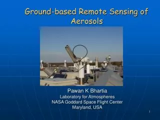
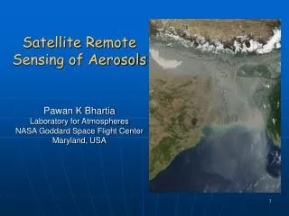
Satellite Remote Sensing of Aerosols. Pawan K Bhartia Laboratory for Atmospheres NASA Goddard Space Flight Center Maryland, USA. Linkages. A Priori information. Ground-based remote sensing. Satellite remote sensing. Laboratory Measurements. In situ field Measurements. Aethalometer

E N D
Satellite Remote Sensing of Aerosols Pawan K Bhartia Laboratory for Atmospheres NASA Goddard Space Flight Center Maryland, USA
Linkages A Priori information Ground-based remote sensing Satellite remote sensing Laboratory Measurements In situ field Measurements • Aethalometer • Nephalometer • Particle Counters • • • • • • • • • Direct-sun • Sky-radiance • Hem. Irradiance • Lidar • Solar occultation • Solar backscattered • Lidar • Chemical prop • Optical prop • Particle shape ISSAOS 2008
Outline • Basic Concepts • Solar Occultation/ Limb scattering • Multi-spectral backscattered radiance • Multi-angle backscattered radiance • Polarization • Satellites/Instruments • The “A-train” • MODIS, MISR & OMI • Model comparisons ISSAOS 2008
Solar Occultation & Limb Scattering Limb Scatt: measures Laer,throughout the orbit, but much less accurate than occultation. Occultation: measures text, sunrise & sunset only, twice per satellite orbit Both methods limited to the stratosphere because of cloud interference ISSAOS 2008 Ref: www-sage2.larc.nasa.gov/ www.iup.uni-bremen.de/sciamachy/
A typical scene from a nadir-viewing satellite instrument ISSAOS 2008
Backscattered Radiance Method I0 L Backscattered radiance (watt/m2/nm/sr): L(q0,q,f0-f) Top-of-the-atm Reflectance: r(q0,q,f0-f) =pL/I0cosq0 Surface reflectance: rs(q0,q,f0-f) q0 q • can be thought ofas the Lambert-eqv reflectivity of the atmosphere. A Lambertian surface of reflectivity r will produce radiance L in the direction (q0,q,f0-f). ISSAOS 2008
Properties of TOA Reflectance (r) r=rRayl+raer+TRaylTaerrs+ …. higher order terms inaccessible by satellite Phase fn is small For satellites, typically, raer=0.1taer Therefore, to get ±0.05 precision in estimating taer one needs ±0.005 precision in estimating rs. ISSAOS 2008
Reflectivity of Ocean rs(q0,q,f0-f)=rFresnel+rwater-leaving+rwhite_caps Solar glint q0 q • Fresnel Reflection: • q0=q and f0-f=180˚ • independent of l • cone angle depends upon wind speed. • diffuse (l-dep) sky radiance is Fresnel reflected at all angles. • Water Leaving Radiance: • strongly l-dep, peaks at ~400 nm. Very small >500 nm. • reduced by chlorophyll and CDOM absorption, enhanced by sediments. • weak angular dependence. • White Caps: • important at high wind speeds only ISSAOS 2008
Remote Sensing of Aerosols over open ocean AVHRR Channel 1 (0.6 mm) Ocean reflectivity at l>0.5 mm is very small at directions away from the solar glint direction, which allows accurate estimation of AOT from satellites Over most of the open ocean, cloud contamination is the main error source. UV/blue ls are much less suitable over ocean. ISSAOS 2008
Estimation of size distribution from l-dependence of s or t wt fns 2m l= 0.34 • s is sensitive to a limited range of particle volumes • As W moves to right with increase in l, itsamples larger particles issue: W is very sensitive to REAL(m), which varies significantly. ISSAOS 2008
Aerosol Remote Sensing Over Land Land reflectivity is larger and highly variable, both spectrally and with viewing geometry, which makes it difficult to do aerosol remote sensing over land. Several clever techniques have been devised to minimize the problem. ISSAOS 2008
Why can’t one see aerosols over bright surfaces? r=rRayl+raer+TRaylTaerrs+… • Since aerosols reflect light to space, as raer increases Taer decreases. This reduces the effect of aerosols when rs≠0. • At some surface reflectivity (rs), 2nd and 3rd terms can cancel, i.e., aerosols cannot be seen at all. • If aerosols are absorbing, they can decrease r over bright surfaces. Dust storm over the Red Sea ISSAOS 2008
Land Aerosols Techniques • Operational MODIS technique • In near IR r≈ rs for small particles • At other ls, estimate rs(l)=k(l)rs(IR), where k(l) are pre-tabulated • “Deep Blue” Technique • Takes advantage of the fact that deserts appear dark at blue wavelengths • Multi-angle Technique r=rRayl+raer+TRaylTaerrs+ …. ISSAOS 2008
Multi-angle Technique Satellite motion Because of the cosq term, raer becomes at large large q, hence surface contribution becomes smaller. P(Q) also changes with Q providing phase fun information to help select the correct aerosol model to do retrieval. q1 q2 Q1 Q2 ISSAOS 2008
Large Rayleigh scattering makes UV unattractive for measuring aerosol scattering. (At 340 nm rRayl can be 10-20 times larger than raer.) • In UV, aerosol absorption reduces the Rayleigh scattering from below the aerosol layer. This effect can be quite large if the aerosols are elevated. • Chief advantage of UV is that smoke and dust plumes can be detected over both dark and bright surfaces, including clouds, deserts, and snow/ice. • Retrieval algorithms exist to estimate tabs=text(1-w0) over dark surfaces. UV Remote Sensing of Aerosols
Dust OC tabs=0.05 BC How do aerosols absorb in the UV? ISSAOS 2008
blue Solar ZA: 45˚-55˚ Satellite ZA: 0˚-60˚ Azimuth= ~90˚ Solar ZA: 45˚-55˚ Satellite ZA: 0˚-60˚ Azimuth= ~90˚ color Saturation Curve Shifts due to aerosol absorption Sky brightness gray Effect of aerosol absorption on UV reflectance ratio • UV Aerosol Index (UV-AI) is derived from the left-down shift of this curve due to aerosol absorption • The shift is proportional to tabs, but depends upon the height of the aerosol plume, higher the plume larger the shift. ISSAOS 2008
TOMS UV Aerosol Index Smoke Desert Dust Smoke from Colorado fires (June 25, 2002) Transport of Mongolian dust to N. America in April 2001. This image was made by compositing several days of TOMS data. ISSAOS 2008
Older Instruments with Long Time Series AVHRR on NOAA Polar Satellites TOMS on Nimbus-7 Sea-WIFs Eqv. AOT UV-Aerosol Index Dust plume image ISSAOS 2008
2008 2008
Aerosol Instruments on the A-Train • Aqua • Moderate Resolution Imaging Spectroradiometer (MODIS) • Terra (not part of the A-train) • MODIS • Multi-angle Imaging Spectroradiometer (MISR) • Aura • (UV aerosols) Ozone Monitoring Instrument (OMI) • Parasol • Multi-angle polarization measurement. • CALIPSO • Aerosol Lidar ISSAOS 2008
MODerate-resolution Imaging Spectroradiometer [MODIS] • NASA, Terra & Aqua • launches 1999, 2001 • 705 km polar orbits, descending (10:30 a.m.) & ascending (1:30 p.m.) • Sensor Characteristics • 36 spectral bands ranging from 0.41 to 14.385 µm • cross-track scan mirror with 2330 km swath width • Spatial resolutions: • 250 m (bands 1 - 2) • 500 m (bands 3 - 7) • 1000 m (bands 8 - 36) • 2% reflectance calibration accuracy • onboard solar diffuser & solar diffuser stability monitor Improved over AVHRR: • Calibration • Spatial Resolution • Spectral Range & # Bands Source: MODIS Team, NASA/GSFC
MODIS Results AOT Fine to Coarse Mode Fraction ISSAOS 2008
While Indonesia’s smoke had a strong peak in 2006, S. America was more normal. This has a lot to do with wet/dry years and the opposite effects of El Niño on the two regions
MODIS aerosol products used to identify interannual patterns. Slopes of 6 year AOD trend (2000 - 2005) Strong Increase Of smoke In 6 years Sudden Decrease In 2006 Difference Between 2006 And 2005 Decrease due to a combination of a wetter year and small rural farmers adhering to fire control measures Koren et al. (2007)
Multi-angle Imaging SpectroRadiometer • Nine CCD push-broom cameras • Nineviewangles at Earth surface: 70.5º forward to 70.5º aft • Fourspectralbands at each angle: 446,558,672,866 nm • Studies Aerosols, Clouds, & Surface http://www-misr.jpl.nasa.gov
MISR Monthly Global Aerosol Mid-VIS AOT July 2005 • Land & Water • Bright Surfaces • Globe ~ weekly • ~ 10:30 AM [+ particle size, shape, SSA constraints] January 2005
nadir 70º Sensitivity to aerosols over bright surfaces Thin haze over land is difficult to detect in the nadir view due to the brightness of the land surface Saudi Arabia, Red Sea, Eritrea Over Bright Desert Sites, mid-vis. AOT to ±0.07 [Martonchik et al., GRL 2004]
MISR height analysis of World Trade Center plume 12 September 2001 MISR 70º image MISR stereo heights of plume patches From: Stenchikov et al., J. Env. Fl. Mech., 2006
Polarization & Anisotropy of Reflectances for Atmospheric Sciences coupled with Observations from a Lidar (PARASOL) POLDER instrument 6 km x 7 km nadir pixel 9 channels (443-910 nm) 3 polarization channels (443, 670, 865 nm) Best for detecting fine mode fraction and particle shape. //smsc.cnes.fr/PARASOL/
Ozone Monitoring Instrument Joint Dutch-Finish Instrument with Dutch/Finish/U.S. Science Team • PI: P. Levelt, KNMI • Hyperspectral wide FOV Radiometer • 270-500 nm • 13x24 km nadir footprint • Swath width 2600 km 2-dimensional CCD wavelength ~ 780 pixels ~ 580 pixels viewing angle ± 57 deg flight direction » 7 km/sec 13 km (~2 sec flight)) 2600km ISSAOS 2008 12 km/24 km (binned & co-added)
Absorbing Aerosols as seen by OMI Dust Smoke Aerosol Transport across the Oceans in terms of the Absorbing Aerosol Index
Retrieving Aerosol Absorption in the near-UV March 9, 2007 By means of an inversion algorithm AOD and SSA are derived
Alaska/Canada smoke transport • North America Boreal fire • In July 2004, large forest fires occurred in the North America boreal region. Smoke aerosols were being transported to large areas in Canada and the U.S., affecting regional air qualities. • Figures show the aerosol distributions of July 2004 over North America as seem by the MODIS and MISR satellite instruments and simulated by the GOCART model. Superimposed in circle are the aerosol optical depth measured by the AERONET sunphotometer network • NASA data used: MODIS, MISR, AERONET for aerosol optical depth, MODIS fire counts for modeling (Petrenko et al., AMS meeting, 2007).
MODIS, MISR, GOCART, AERONET: 200407 AERONET data in circles AERONET data in circles • Feature: North America Boreal fire – captured by MODIS, MISR, GOCART • MODIS: Not available over bright surfaces (e.g., deserts) and cloudy regions (e.g., N. Pacific) • MISR: Not available over cloudy regions (N. Pacific, central America); excessive AOT over Greenland • GOCART: North America boreal fire emission or injection height maybe too low so smoke did not go far enough AERONET data in circles
Aerosols in 200010 and 200610:North America and Europe: Decrease from 2000 to 2006. East Asia: Increase from 2000 to 2006. Indonesia: Intense fire in October 2006 2000010 MODIS GOCART 2000610 MODIS GOCART
The figures below show global aerosol distribution and transport observed by the MODIS instrument on EOS-Terra (left column) and simulated by the global model GOCART (right column) for April 13 (top row) and August 22 (bottom row), 2001. Red color indicates fine mode aerosols (e.g., pollution and smoke) and green color coarse mode aerosols (e.g., dust and sea-salt). Brightness of the color is proportional to the aerosol optical depth. On April 13, 2001, there are heavy dust and pollutions transported from Asia to the Pacific and dust transported from Africa to Atlantic; while on August 22 large smoke plumes from South America and Southern Africa are evident. Figure credit: Yoram Kaufman. MODIS (Satellite) GOCART (Model)
Trans-Pacific Transport of Dust Dust AOT April 8, 2001 GOCART TOMS AI April 8, 2001 Dust AOT April 11, 2001 GOCART TOMS AI April 11, 2001 Dust AOT April 14, 2001 GOCART TOMS AI April 14, 2001 Simulated by GOCART (model) Observed by TOMS (satellite) Trans-Pacific transport of dust in April 2001. Dust originating from Asian desert (April 8) is being transported across the Pacific and reaches North America (April 14). Left column: GOCART model simulation; right column: aerosol index from NASA satellite instrument TOMS (Chin et al., JGR 2003).
Contribution of Satellites in improving aerosol models • Improving the dust sources by comparing models with TOMS AI (Ginoux et al.). • Mass transport of dust and pollution aerosols using MODIS (Kaufman et. al. 2005) • MISR smoke plume height to improve smoke injection height. • MISR non-spherical particle fraction for evaluating model-derived dust and non-dust aerosols.
Further Reading Nature, Vol 419, 12 Sept 2002 Yoram Kaufman 1948-2006
Passive Remote Sensing of Aerosols by Satellites- Future • New instruments will have MODIS-like spatial and spectral coverage with MISR and PARASOL-like multi-angle and polarization capability to determine ref index, size, and shape. • Advanced UV instruments may allow separation of OC and BC aerosols. • High spectral resolution O2-A band measurements may provide aerosol vert profile information with daily global mapping.
Some Satellite-Aerosol Product Web Sites • http://www-misr.jpl.nasa.govMISR Home page; background, image gallery,.. • http://eosweb.larc.nasa.govMISR, CERES, SAGE, MOPITT, TES, data & docs • http://modis-atmos.gsfc.nasa.gov/IMAGES/index.htmlMODIS global browse imagery • http://g0dup05u.ecs.nasa.gov/Giovanni/MODIS on-line visualization & analysis tools • http://modis-atmos.gsfc.nasa.gov/MODIS atmosphere products & docs • http://cybele.bu.edu/modismisr/index.htmlMISR+MODIS climate data (surface emphasis) • http://modis-fire.umd.edu/ MODIS-UMD Fire products & docs • http://maps.geog.umd.edu/default.asp MODIS-UMD global Fire occurrence mapper • http://idea.ssec.wisc.edu/ IDEA merged MODIS-EPA Air Quality • http://alg.umbc.edu/usaq/ UMBC Air Quality events • http://jwocky.gsfc.nasa.gov/eptoms/ep.htmlTOMS/OMI aerosol & O3, data & docs • http://www.osdpd.noaa.gov/PSB/EPS/Aerosol/Aerosol.html NOAA AVHRR aerosols • http://oceancolor.gsfc.nasa.gov/SeaWiFS/BACKGROUND/SeaWiFS data & docs • http://aeronet.gsfc.nasa.gov/AERONET AOT & properties, data & docs
Levy et al., 2nd generation MODIS Land algorithm, JGR, vol 112, (doi:10.1029/2006JD007815 & 10.1029/2006JD007811), 2007.