Download
1 / 1
10 likes | 101 Vues
This study presents a new approach to climate forecasting using fractal analysis, considering long-term self-similarities in climate data. The research explores the non-linear behavior of global climate patterns and provides 25-year forecasts for California, Kansas, and Texas. By employing fractional differencing models, the study predicts temperature, precipitation, and drought severity indices in the southwestern United States. The findings suggest that global weather patterns exhibit a warming trend followed by a downward shift, with different regions experiencing varied recovery periods. Understanding the fractal nature of climate data can lead to more accurate forecasts and tailored policies.

E N D
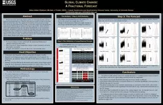
Global Climate Change: A Fractional Forecast Akbar Akbari Esfahani, Michael J. Friedel, USGS - Crustal Geophysics and Geochemistry Science Center, University of Colorado Denver aesfahani@usgs.gov, mfriedel@usgs.gov Abstract The Analysis – Step 1: Self-Similarity Step 3: The Forecast • The climate data presented here are self-similar. [5] • So we only present one sample data set.[5] • Changes in the Information Dimension imply changes in the entropy and therefore point to changes in trends.[2] Below are 25 year forecasts of climate parameters (PDSI, Precip, and Temp) for California, Kansas, and Texas. The plots display time series [1], forecast, and standardized residuals. We have previously shown that climate variables are self-similar in nature, and thus represent long-memory processes. Therefore, these processes need to account for fractional differences in the time series. This requires that we make use of fractal analysis in time series and use fractional differencing. To begin, it is possible to make short term predictions using fractional differencing auto-regressive moving-average models, which can then be used to make appropriate policies for each region. For predictions, we use reconstructed temperature, precipitation, and Palmer Drought Severity Index data of the southwestern United States (US). It is important to note that the global climate patterns are not on a linear scale but rather behave non-linear on a multi-scale pattern and thus we cannot just use the ordinary toolset given by statistic and time series analysis. These findings provide a different view of climate change for the coming years in the US. California Precip Forecast California PDSI Forecast Standardized residuals Standardized residuals Standardized residuals California Temp Forecast California Temp California Precip California PDSI Information Dimension Information Dimension Information Dimension Kansas Temp Forecast Kansas Precip Forecast Standardized residuals Kansas PDSI Forecast Standardized residuals Standardized residuals Problem Time in 25 year Intervals Time in 25 year Intervals Time in 25 year Intervals Step 2: The Validation of Long-Memory Process • To forecast climate we must understand the underlying Mathematical structureof the given time-series. • Most forecasts of future temperature change assume stationarity and more importantly, seasonality. • To apply self-similarity to forecast that is not a seasonal time series. • A valid FARIMA forecast requires existence of a long-memory process. [6] Hurst Parameters for Long-Memory Process Goal\Objective Standardized residuals Texas Precip Forecast Standardized residuals Texas PDSI Forecast Standardized residuals Texas Temp Forecast California PDSI Differencing • Understand scale-dependent relations among derived climate variables. • Quantify fractal dimension and evaluate spatial nature of self similarity for temperature, precipitation, Palmer Drought Severity Indices in various states of the USA. • Quantify fractional differenced information and evaluate spatial climate shocks using the fractal information dimension number for various states of the USA. • Use the quantified fractal information to make accurate forecasts. As H (Hurst Parameter) approaches 1, the more persistent the time series becomes. If there is no long-memory effect, H = 0.50. [6] A zero autocorrelation of residuals suggests white noise and correct use of time-series parameters. California Precip Differencing • From the plots we observe that a higher PDSI corresponds to a higher Precipitation rate and lower temperatures and vice versa, which follows the expected pattern for the Palmer Drought Severity Index. Methodology Long-Memory Parameter, λ. For Long-Memory 0 < λ < 1. Conclusions We employ fractal analysis to study the temporal self similarities of climate data: We evaluate climate data over 2000 years. [1] Climate data is split into 25 year intervals. [3] Climate fractal Dimensions. [6] Table 1: Calculation of PDSI (Palmer Drought Severity Index), Temp (Temperature) and Precip (Precipitation, [mm]) data [1], [4]: [3] Use a Fractional Auto-Regressive Differenced Moving-Average (FARIMA) model to forecast.[6] • Our global weather patterns seem to be reaching the peak of a warming period (or have reached it in some places) and are now approaching a downward trend for temperature. • The residuals are normally distributed indicating our forecast model is unbiased. • A dry period will be followed by a wet period. However, to reach that equilibrium, each region has a different time period of recovery. • The global warming that we are currently experiencing, in certain parts of the world, is the system recovery period needed to reach equilibrium from the Little Ice Age, which ended around the turn of the 20th century. • Each region behaves differently in regards to the coming changes; thus, the regional forecasts (and local forecasts) can help land and water managers with their decision making. • It is important that we relate weather changes not only on a global scale, but also to a temporal scale long enough that can give scientists a bigger picture. More importantly we have to be mindful that our global weather patterns are on a non-linear spatial temporal scale that change on a local scale first and then on larger scale. California Temp Differencing As λ (long-memory parameter) approaches 0, the more pronounced is the long-memory. [6] The more Fractional the numbers the more exact the Self-Similarity and a stronger Fractal Nature. References [1] Friedel, M. J. ( in press). Climate change effects on ecosystem services in the United States – issues of national and global security, In: Baba, A., Chambel, A., Friedel, M.J., Haruvy, N., Howard, K.W.F., and Raissouni, B., (eds), 2010. Climate change and its effect on water supplies - Issues of National and Global Security, NATO Science Series, IV. Earth and Environmental Sciences – vol. xx, Springer, Dordrecht, The Netherlands [2] Daniel Barbara. Chaotic Mining: Knowledge Discovery Using the Fractal Dimension, George Mason University, Information and Software Engineering Department, Fairfax, VA [3] Plots and data analysis was performed with R. “R-project.com” using the package fdim, by: Fco. Javier Martinez de Pison Ascacibar, et all, Functions for calculating fractal dimension, [4] Cook, E.R., & Woodhouse, C.A., Eakin, C.M., Meko, D.M., and Stahle, D.W. (2004). Long-Term Aridity Changes in the Western United States. Science, 306(5698):1015-1018.\ [5] Akbari Esfahani, A., & Friedel, M.J. (2010). Understanding Global Climate Change: A Fractal View [Abstract]. American Geophysical Union Meeting 2010, San Francisco. [6] Beran, Jan (1998). Statistics for Long-Memory Processes. New York, NY: Chapman & Hall/CRC.