Global Ice Sheet Interferometric Radar
Global Ice Sheet Interferometric Radar. NASA ESTO IIP Ohio State Univ., JPL, Univ. Kansas, VEXCEL Corp., E.G&G Corp., Wallops Flight Facility. GISIR Instrument. GISIR mid-year review Science Spaceborne Instrument Concept Strawman Design Simulations Aircraft Experiment Management

Global Ice Sheet Interferometric Radar
E N D
Presentation Transcript
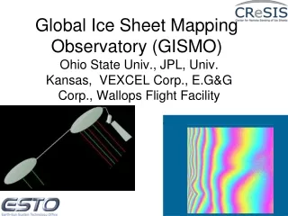
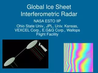
Global Ice Sheet Interferometric Radar NASA ESTO IIP Ohio State Univ., JPL, Univ. Kansas, VEXCEL Corp., E.G&G Corp., Wallops Flight Facility
GISIR Instrument • GISIR mid-year review • Science • Spaceborne Instrument Concept • Strawman Design • Simulations • Aircraft Experiment • Management • GISIR Team • K.Jezek, E. Rodriguez, P. Gogineni, J. Curlander, X. Wu, J. Sonntag, W. Krabill, P. Kanagaratnam, C.Allen, A. Freeman. T. Akins • D. MacAyeal, R. Forster, S. Tulazek, M. Fahnestock, S. Clifford
Glaciers and Ice Sheets ‘Grand Challenges’ • Understand the polar ice sheets sufficiently to predict their response to global climate change and their contribution global sea level rise • What is the mass balance of the polar ice sheets? • How will the mass balance change in the future?
Reservoirs of Fresh Water Fresh Water Resource Polar Ice Sheets and Glaciers 77% East Antarctica 80% West Antarctica 11% Greenland 8% Glaciers 1% Ice Thickness Average: 2500m Maximum: 4500m National Geographic Magazine
Glacier/Ice Shelf Change • In last 4 years, numerous observations of glacier/ice shelf reduction • Interior Antarctic Peninsula glaciers (Scambos, 2004) • Larsen ice shelf (many) • Jacobshaven glacier in Greenland (Thomas, 2003) • Pine Island and Thwaites (Rignot, 2001) • None of these observations are predicted by climate models 1963-1997 0.8% decrease in Ice Shelf extent between 1963 and 1997 Kim and Jezek
Mass Balance • Ice sheet mass balance is described by the mass continuity equation Altimeters Act/Pass. Microwave InSAR No spaceborne technique available Evaluations of the left and right hand sides of the equation will yield a far more complete result
Ice Dynamics and Prediction Force Balance Equations No Sat. Cover Satellite Altimetry Basal Drag, Inferred at best Terms related to gradients in ice velocity (InSAR) integrated over thickness Understanding dynamics coupled with the continuity equations yields predictions on future changes in mass balance
Glaciers and Ice Sheets Mapping Orbiter • Key Measurements: • Determine total global volume of ice in glaciers and ice sheets • Map the basal topography of Antarctica and Greenland • Determine basal boundary conditions from radar reflectivity • Map internal structures (bottom crevasses, buried moraine bands, brine infiltration layers)
Measure ice thickness to an accuracy of 20 m or better Measure ice thickness every 1x1 km (airborne < 250 m) Measure ice thickness ranging from 100 m to 5 km Measure radar reflectivity from basal interfaces (rel. 2 dB) Obtain swath data for full 3-d mapping Measure internal layers to about 20 m elevation accuracy Pole to pole observations; ice divides to ice terminus One time only measurement of ice thickness Repeat every 5-10 years for changes in basal properties Global Ice Sheet Mapping Orbiter Prioritized Science Requirements
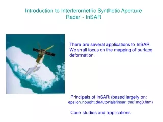
A New Technical Approach Required • Nadir sounding ‘profiler’ cannot meet science requirements: • Beam limited cross-track spatial resolution (1km) requires antenna size beyond current capabilities (420 m at P-band) • Available bandwidth (and range resolution) insufficient for desired 10m height accuracy: 6Hz gives a range resolution of 13.8 m in ice. Worse at VHF • Full spatial coverage requires years of mission lifetime (high costs)
Other Conventional Approaches Limited • Conventional Interferometry is Insufficient • Coverage, spatial resolution, and height accuracy suggest a swath SAR interferometer might meet concept • Ambiguous returns from surface clutter and the opposite side basal layer make this approach not feasible • An alternate approach: multiple baselines to resolve subsurface/surface, expensive and hard to implement: • Minimum of 3 antennas are required to get necessary baselines • The technique is sensitive to calibration and to SNR • Data rate is high
Primary Technical Challenge Surface Clutter • Separate basal return from surface clutter Weak Echos Strong Attenuation
Interferometric Sounding Concept • Conventional interferometry uses phase information one pixel at a time • Additional information contained in the spatial frequency of the phase: • Because of the difference in incidence angles, the near nadir interferometric phase spatial frequency from the basal return is much larger than the equivalent frequency for surface clutter • Opposite side ambiguities have opposite interferometric frequencies: while the phase in one side increases with range, it decreases with range in the opposite side (+/- spatial frequencies of complex interferogram) • IFSAR sounding concept: spatially filter interferogram to retain only basal returns from one side Satellite height (H); ice surface height (h); Depth of the basal layer (D); topographic variations of the basal layer (d); cross-track coordinate of the basal layer point under observation (xb); and, xs is the cross-track coordinate of the surface point whose two-way travel time is the same as the two-way travel time for xb.
Interferometric Phase and Phase Frequency Complex interferogram Surface interferometric phase difference Basal interferometric phase difference Surface interferogram slope as a function of range. hx is the surface topography cross-track slope Basal Interferogram slope as a function of range. dx is the basal topography cross-track slope (From E. Rodriguez, 2004)
Surface vs Basal Cross-Track Distance Surface cross-track distance xs as a function of basal cross-track distance xb for a platform height of 600km. Notice that near nadir xs is nearly independent of xb, while for xb > 50 km, the two are close to being linearly dependent.
Fringe Spectrum • Interferogram spectra for • first 50 km of xb • - signal to clutter ratio - 1 • - radar freq - 430 MHz • - bandwidth of 6 MHz • Basal spectrum is • colored orange • Surface spectra for • - D = 1 km (black), • - D = 2 km (red), • - D = 3 km (green), • - D = 4 km (blue). • Note the basal fringe • spectrum depends very • weakly on depth
Clutter Effect on Interferometric Error Height error as a function of signal to clutter (a/b) for a baseline of 45 m and a center frequency of 430~MHz (solid lines) and 130 MHz (dashed lines). The values of (a/b) are: 0 dB (black), -10 dB (red), and -20 dB (blue).
Height Noise vs SNR Height error as a function of SNR for a baseline of 45m and a center frequency of 430 MHz (solid lines) and 130 MHz (dashed lines). The values of SNR are: 0 dB (blue), -5 dB (red), and -10 dB (black). The number of looks is assumed to be 100.
Height Error After Interferometric Filtering: 45m Baseline Assumed clutter to signal ratio (same side): 0dB Assumed clutter to signal ratio (opposite side): -3dB Assumed SNR: 0dB Assumed number of spatial looks: 100
Desired Swath/Altitude • A 50 km swath will enable a mission lifetime < 4 months • A 50 km swath is consistent with the interferometric sounder approach for a height of 600 km and a 6 MHz bandwidth • Heights lower than 600 km will require a decrease in swath and a consequent increase in mission lifetime (although this is not a strong constraint)
Radar Frequency Selection • Select P-band (430MHz) to minimize baseline length, antenna size and range resolution • Antenna length of 12.5 m consistent with demonstrated space technology (TRL 9) • Baseline range between 30m to 60m consistent with SRTM mast (TRL9) • 6MHz bandwidth possible at P-band • Higher clutter mitigated by interferometric sounder technique • VHF only feasible using repeat pass interferometry, although antenna size (~40m) may be problematic. • Can 1 MHz remote sensing band be increased over the polar regions?
Pulse Length Selection • In order to minimize contamination from nadir surface return, use short 20usec chirp • surface nadir return sidelobes stops after 1.7 km of ice depth • Much longer pulses will contaminate basal returns significantly
PRF Selection • Required PRF for SAR synthetic aperture: ~1KHz • Use significantly higher PRF (~7KHz - 10KHz) together with onboard presum to improve signal to noise ratio • Instrument duty cycle: ~20%
Mission Concept • P-band (430 MHz), 6 MHz bandwidth • attenuation is essentially same at from 100 MHz to 500 MHz • along-track resolution from SAR processing • cross-track resolution from pulse bandwidth • Two antennas, 45 m baseline, off-nadir boresight - 1.5 degrees • mesh dishes, SRTM-like boom, 50 km swath from 10 to 60 km cross-track • use conventional nadir sounding for layering studies • Fully polarimetric for ionospheric effects • 600 km altitude, 1 year minimum mission lifetime
Key Instrument Parameters Polarimetric 4 channels Center frequency 430 MHz Bandwidth 6 MHz Pulse length 20 ms Peak transmit power 5 kW System losses -3 dB Receiver noise figure 4 dB Platform height 600 km Azimuth resolution 7 m PRF 10 kHz Duty cycle 20 % Antenna length 12.5 m Antenna efficiency -2. dB 1-way Antenna boresight angle 1.5 deg Wavelength 0.7 m Baseline 45 m Swath 50 km Minimum number of looks 500
Assumed Antenna Pattern • Assume uniform circular illumination • Antenna diameter 12.5m • consistent with available space qualified antennas • Antenna boresight: 1.5deg • Assumed antenna efficiency: -2dB 1-way
Model Backscatter Cross Section • The backscatter model consists of two contributions: • Geometrical optics (surface RMS slope dependent) • Lambertian scattering • assumed Lambertian contribution at nadir: -25dB
Observed Surface Sigma0 Angular Dependence at 120 MHz • Data obtained with the JPL Europa Testbed Sounder in deployment with the Kansas U. sounder over Greenland • Angular decay near nadir (>15 dB in 5 degrees) consistent with very smooth ice surface • Change in behavior at P-band is still unknown, but probably bounded by 1-3 degree slope models
Estimated One-Way Absorption Absorption losses present severe constraints on system design if an SNR > 0dB is desired. Together with pulse length considerations, this leads to a desired peak power of ~5kW, which is technologically feasible at P-Band
Phase History Simulation • DEM for surface and basal region from Greenland • Assume homogeneous ice volume • permittivity3.4 for ice, 9 for bedrock • intermediate layers are weakly scattering at off-nadir angles • Attenuation 9 dB/km • Ice thickness 2.0 to 2.5 km • Process: create reflectivity map of surface and subsurface • Construct phase history data (PHD) using inverse chirp scaling • Process PHD with COTS SAR processor and interfeometric processor to 80 looks
Key instrument and geometry parameters • Platform Height: 600 km • Center Frequency: 430 MHz • Chirp Bandwidth: 6 MHz • Pulse Length: 20 us • PRF: 2 kHz • Antenna Length: 12.5 m • Antenna Boresight Angle: 1.5o • Baseline: 45 m
148.8 km (ground range) 148.8 km DEMS in slant range geometry echo delay caused by the ice thickness at nadir 137.5 km (b) basal DEM (a) surface DEM
Simulation Results for GISMO surface and basal interferogram original ice thickness +2500 m Error is 0 to 20 m out to 50 Km +2137 m Derived ice thickness (expected performance reduction pass 50 km) Band-pass filtered interferogram +2850 m +1714 m Images are 130 km vertical (azimuth and 70 km ground range (11.9 km slant range)
Interferogram range spectrum The peak near 0 frequency represents the surface contribution and the peaks at the right side are from base contribution.
Airborne SAR processor • Modify Vexcel’s current fast-back-projection space-borne spotlight SAR processor to be able to process the simulated airborne stripMap SAR data
Modifications for airborne simulation • Airborne platform with air turbulence • Varying PRF • Interferometric mode with 2+ receiving antennas • Inverse chirp-scaling modifications for varying PRF and sensor velocity • Airborne SAR processor
Scaling GISMO to Aircraft Altitudes • Preserve the fringe rate separations: Find that basal distance for comparable fringe separations scale as the square root of the platform hieghts: 600km elevation satellite imaging a swath from 10 km to 60 km corresponds to aircraft at 6 km imaging 1 to 6 km. • Preserve number of fringes: imposes a restriction on the baseline. 45 m spaceborne baseline means a 4.5 m baseline on aircraft. 10 to 20 m better. • Maintain geometric correlation: Limiting phase change over a resolution cell imposes a restriction on bandwidth. Find 45-90 MHz depending on baseline. Larger bandwidth also preserves number of samples per swath • Achievable with P-3; on the edge with Twin Otter