Looking at data: relationships Least-squares regression
250 likes | 450 Vues
Looking at data: relationships Least-squares regression. IPS chapter 2.3. © 2006 W. H. Freeman and Company. Objectives (IPS chapter 2.3). Least-squares regression The regression line Making predictions: interpolation Coefficient of determination, r 2 Transforming relationships.

Looking at data: relationships Least-squares regression
E N D
Presentation Transcript
Looking at data: relationshipsLeast-squares regression IPS chapter 2.3 © 2006 W. H. Freeman and Company
Objectives (IPS chapter 2.3) Least-squares regression • The regression line • Making predictions: interpolation • Coefficient of determination, r2 • Transforming relationships
Correlation tells us about strength (scatter) and direction of the linear relationship between two quantitative variables. In addition, we would like to have a numerical description of how both variables vary together. For instance, is one variable increasing faster than the other one? And we would like to make predictions based on that numerical description. But which line best describes our data?
Distances between the points and line are squared so all are positive values. This is done so that distances can be properly added (Pythagoras). The regression line The least-squares regression line is the unique line such that the sum of the squared vertical (y) distances between the data points and the line is the smallest possible.
is the predicted y value (y hat) b is the slope a is the y-intercept Properties The least-squares regression line can be shown to have this equation: "a" is in units of y "b" is in units of y / units of x
How to: First we calculate the slope of the line, b; from statistics we already know: r is the correlation. sy is the standard deviation of the response variable y. sx is the the standard deviation of the explanatory variable x. Once we know b, the slope, we can calculate a, the y-intercept: where x and y are the sample means of the x and y variables This means that we don't have to calculate a lot of squared distances to find the least-squares regression line for a data set. We can instead rely on the equation. But typically, we use a 2-var stats calculator or stats software.
BEWARE!!! Not all calculators and software use the same convention: Some use instead: Make sure you know what YOUR calculator gives you for a and b before you answer homework or exam questions.
Software output intercept slope R2 r R2 intercept slope
They are NOT points from your sample data (except by pure coincidence). The equation completely describes the regression line. To plot the regression line you only need to plug two x values into the equation, get y, and draw the line that goes through those those points. Hint: The regression line always passes through the mean of x and y. The points you use for drawing the regression line are derived from the equation.
Hubble telescope data about galaxies moving away from earth: These two lines are the two regression lines calculated either correctly (x = distance, y = velocity, solid line) or incorrectly (x = velocity, y = distance, dotted line). The distinction between explanatory and response variables is crucial in regression. If you exchange y for x in calculating the regression line, you will get the wrong line. Regression examines the distance of all points from the linein the y-direction only.
Correlation versus regression The correlation is a measure of spread (scatter) in both the x and y directions in the linear relationship. In regression we examine the variation in the response variable (y) given change in the explanatory variable (x).
Nobody in the study drank 6.5 beers, but by finding the value of from the regression line for x = 6.5 we would expect a blood alcohol content of 0.094 mg/ml. Making predictions: interpolation The equation of the least-squares regression allows to predict y for any xwithin the range studied. This is called interpolating.
= - ˆ y 0 . 125 x 41 . 4 = - ˆ y 0 . 125 x 41 . 4 (in 1000’s) There is a positive linear relationship between the number of powerboats registered and the number of manatee deaths. The least squares regression line has the equation: Thus if we were to limit the number of powerboat registrations to 500,000, what could we expect for the number of manatee deaths? Roughly 21 manatees.
!!! !!! Extrapolation Extrapolation is the use of a regression line for predictions outside the range of x values used to obtain the line. This can be a very stupid thing to do, as seen here. Height in Inches Height in Inches
Example: Bacterial growth rate over time in closed cultures If you only observed bacterial growth in test-tube during a small subset of the time shown here, you could get almost any regression line imaginable. Extrapolation = big mistake.
The y intercept Sometimes the value of the y-intercept is not biologically possible. Here we have negative blood alcohol content, which makes no sense… y-intercept shows negative blood alcohol But the negative value is appropriate for the equation of the regression line. There is a lot of scatter in the data, and the line is just an estimate.
Coefficient of determination, r 2 r 2 representsthe percentage of the variance in y(vertical scatter from the regression line) that can be explained by changes in x. r 2, the coefficient of determination, is the square of the correlation coefficient.
r = 0.87 r2 = 0.76 Changes in x explain 0% of the variations in y. The value(s) y takes is (are) entirely independent of what value x takes. r = 0 r2 = 0 Here the change in x only explains 76% of the change in y. The rest of the change in y (the vertical scatter, shown as red arrows) must be explained by something other than x. r = -1 r2 = 1 Changes in x explain 100% of the variations in y. Y can be entirely predicted for any given value of x.
r =0.9 r2 =0.81 There is quite some variation in BAC for the same number of beers drunk. A person’s blood volume is a factor in the equation that was overlooked here. r =0.7 r2 =0.49 We changed number of beers to number of beers/weight of person in lb. • In the first plot, number of beers only explains 49% of the variation in blood alcohol content. • But number of beers / weight explains 81% of the variation in blood alcohol content. • Additional factors contribute to variations in BAC among individuals (like maybe some genetic ability to process alcohol).
Grade performanceIf class attendance explains 16% of the variation in grades, what is the correlation between percent of classes attended and grade? 1. We need to make an assumption: attendance and grades are positively correlated. So r will be positive too. 2. r2 = 0.16, so r = +√0.16 = + 0.4 A weak correlation.
Transforming relationships A scatterplot might show a clear relationship between two quantitative variables, but issues of influential points or non linearity prevent us from using correlation and regression tools. Transforming the data – changing the scale in which one or both of the variables are expressed – can make the shape of the relationship linear in some cases. Example: Patterns of growth are often exponential, at least in their initial phase. Changing the response variable y into log(y) or ln(y) will transform the pattern from an upward-curved exponential to a straight line.
Exponential bacterial growth In ideal environments, bacteria multiply through binary fission. The number of bacteria can double every 20 minutes in that way. 1 - 2 - 4 - 8 - 16 - 32 - 64 - … Exponential growth 2n, not suitable for regression. log(2n) = n*log(2) ≈ 0.3n Taking the log changes the growth pattern into a straight line.
Body weight and brain weight in 96 mammal species r = 0.86, but this is misleading. The elephant is an influential point. Most mammals are very small in comparison. Without this point, r = 0.50 only. Now we plot the log of brain weight against the log of body weight. The pattern is linear, with r = 0.96. The vertical scatter is homogenous → good for predictions of brain weight from body weight (in the log scale).