Earth Surface Temperature Analysis: Satellite Remote Sensing and Considerations
20 likes | 214 Vues
Earth Surface Temperature Analysis: Satellite Remote Sensing and Considerations. Anderson Valencia, Yassine Mhandi, Yusef Esa, Undergraduate Researchers : LaGuardia Community College

Earth Surface Temperature Analysis: Satellite Remote Sensing and Considerations
E N D
Presentation Transcript
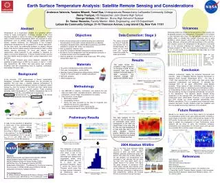
Earth Surface Temperature Analysis: Satellite Remote Sensing and Considerations Anderson Valencia, Yassine Mhandi, Yusef Esa, UndergraduateResearchers: LaGuardia Community College Reina Trumpet, HSResearcher: John Bowne High School George Vaitsos, HS Mentor: Bronx High School of ScienceDr. Yasser Hassebo, Faculty Mentor: Math, Engineering, and CS Department LaGuardia Community College: 31-10 Thomson Avenue, Long Island City, New York 11101 Volcanoes Abstract Volcanoes affect the climate as the ash plume of the eruption can be globally spread to the atmosphere. The position of the volcano is very important also since the high latitude volcanoes have a smaller effect in climate than tropical volcanoes due to arctic oscillation, which doesn’t permit the wide spread of the ash plume. Although, volcanoes emit high quantities of CO2 and SO2, their eruption causes the temperature of the planet to cool down due to the aerosols reflecting the sunlight. For instance, Mt Pinatubo erupted in 1991 and reduced the temperature of Earth by 0.5 oC and some of its pyroclastic flow kept heat for a few years after explosion Temperature, as a biophysical variable, is a powerful variable critical to many investigators. Scientists consider it the most important variable to define the state of the atmosphere. Global maps of Earth Surface Temperature (EST) are required for many applications such as climate change research, global warming studies, weather prediction, etc. Performing in situ (in-place) temperature measurement for the global EST is almost impossible. On the other hand, the relationship between an object’s internal kinetic heat and its radiant energy (external energy) help to utilize remote sensing technology for most real objects. Such relationships, allow scientists to use satellites to measure an object’s true kinetic temperature. Thermal infrared remote sensing has been widely used to measure earth surface temperature from satellites. In this project, students were given datasets, collected from satellites of global maps of EST for six years. A total of 17,520 files representing 181 million real data points was provided. Students used two programming tools to organize, summarize, and analyze the given data. Objectives Data Correction: Stage 3 The areas bounded by lines of longitude and latitude are not divided equally. As a result, as you move from the equator toward the poles the areas get smaller. • Build a strong background of remote sensing and understand • the procedure of how earth surface temperature is collected. • Strengthen Students’ skills in MATLAB programming and SPSS • software to analyze 181 million real data points • Pick up students’ research skills • Study the correlation between temperature and precipitation. • Be able to find the temperature and the precipitation amounts of • a certain location from the available data. • Improve students’ non-academic skills (team work, PPT, writing • and present report, etc.) Figure 6: Taking the areas into consideration because Earth’s grid is not divided into equal areas Figure 12: Data from GISS demonstrates the change of Earth’s monthly temperature after the eruption of Mount Pinatubo. Results Materials The graph shows the progress in data correction for the year of 2004. As we proceed from raw data analysis to the last stage of data correction, the obtained average EST agrees with NOAA’s result . • Six years of temperature profile (2000-2005) • One year of precipitation profile (2004) • National Oceanic Atmospheric Administration (NOAA) results for the same years to validate calculations • MATLAB program • SPSS Statistical tool Conclusion Background • Students understood, deeply, the essential theoretical and scientific ideas of Satellites Remote Sensing techniques to measure Earth Surface Temperature (EST). The total of 17,520 files representing 181 million real data points were organized, summarized, and analyzed to calculate the averaged EST for six years (2000-2005) using Matlab program.. Three stages of data corrections were applied to analyze the EST data: (1) determining and eliminating Outliers, (2) Interpolating Outliers, and (3) Taking the variation of areas, that bounded by the lines of longitude and latitude, into account in the calculations. The research results showed strong agreement, of the average EST, with NOAA’s results for four consecutive years (2002-2005). However, in the years 2000 and 2001 though our values deviated substantially from NOAA’s calculations. This is a potential point requiring further research and work. Finally, students meet the academic and the non-academic learning objectives of the research. In-situ accurate EST measurement is almost unattainable. Nowadays, accurate EST measurement can be provided by satellites. But how does a satellite measure temperature? A satellite doesn’t measure temperature directly. It measures radiant energy Eradfrom the surface of the Earth and then sends those measurements back to the ground stations. There scientists calculate radiant temperature Trad (Earth’s temperature due to its radiant energy) from Erad using Boltzmann’s thermal law Erad = σ·Trad4 and then convert Trad to Ttrue (EST due to its internal energy) using Kirchhoff’s thermal law Ttrue = ε-1/4 Trad Figure 7: Data correction: 3 stages of 2004 temperature profile Methodology • Use MATLAB to organize, summarize, and analyze the raw data and obtain mean, standard deviation, skewness, kurtosis, histograms, contour maps, and determine the outliers. • Data correction: three stages • Eliminating Outliers. • Interpolating Outliers. • Taking the area bounded by the lines of longitude and latitude into account in calculations • Use Statistical software SPSS to verify results. • Verify our research results using NOAA/NASA data Future Research Figure 8: Comparison of our results with NOAA for 6 years (2000-2005) Based on our results, part of our future work is to re-analyze the temperature profile of the years 2000 and 2001 including a fourth stage of correction which is the emissivity impact on the EST profile. Another part will be to use Fourier analysis on our data to explain the propagation of heat. Furthermore, more analysis will be done to verify the correlation between temperature and precipitation for all given years and use that as a possible fifth correction stage of our data. Preliminary Results Figure 1: The procedure of how satellites collect data of temperature measurements The data analysis for the month of July 04 discovered an unforeseen value, which corresponds to the dark red circled area in the map (Fig 9). The very high temperature of that area was due to the 2004 Alaska's massive wildfire. Wildfires are among the most significant ecological effects of climate warming. In order for the scientists to determine in which part of the electromagnetic spectrum Earth radiates energy, Wien's Thermal law is used. According to Wien’s law, λmax = b/T , if we substitute T for the Earth’s mean surface temperature (300 K) we get a λmax of 10.3μm, which falls in the infrared portion of the EM spectrum. Outliers Figure 2: The visible and infrared portion of the EM spectrum Figure 9: Contour map of July 2004 EST Figure 4: Eliminating vs. interpolating outliers Figure 3: Temperature analysis of the first 3 hours of July 2004 2004 Alaskan Wildfire “Two of the three most extensive wildfire seasons in Alaska’s 50-year record occurred in 2004 and 2005” (ACCAP). Wildfires generate greenhouse gases and aerosol that effect the climate globally. In the last decades, the temperatures have increased in high latitudes that can affect the near north pole region which has a greater impact in the climate. That region has great amounts of permafrost which holds carbon dioxide and methane which can be released to the atmosphere with the fires. Although, permafrost is melting due to high temperatures, wildfires will increase the lose of permafrost through the region. The histogram of raw data, figure 3, shows a distribution error which is due to the outliers. The outliers were eliminated and replaced with interpolated values using MATLAB software, figure 4. As a result, the new generated histogram, figure 5, satisfy the Central Limit Theorem, which states that for large number of elements all distributions tend to become a normal. Figure 13: Correlation between temperature and precipitation in 2004 Figure 14: Precipitation map of January 2004 with a “noise” effect outside the 50o N and 50o S area of the Earth References Sponsors: National Aeronautics and Space Administration (NASA) NASA Goddard Space Flight Center (GSFC) NASA Goddard Institute for Space Studies (GISS) NASA New York City Research Initiative (NYCRI) Department of Education - The Alliance for Continuous Learning Environments in STEM (CILES) grant # P031C110158 LaGuardia Community College (LAGCC) Acknowledgements: Dr. William Rossow, Distinguished Professor, EE dept, CCNY Dr. Jorge Gonzalez, ME Professor, PI of CILES grant, CCNY www.nasa.gov www.mathworks.com www.earthobservatory.nasa.gov www.noaa.gov www.universetoday.com http://ine.uaf.edu/accap/research/season_fire_prediction.htm E. Kasischke1 and M. Turetsky, Recent changes in the fire regime across the North American, Geophysical Research Letters , Vol. 33, L09703, 2006 Figure10: Alaska's 2004 Wildfire Figure11: Decrease of permafrost Figure 5: Interpolating outliers 2004 Data Correction: Stage 2