Download
1 / 23
230 likes | 373 Vues
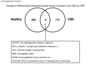
Identifying Differentially Expressed Genes in Unreplicated Multiple-Treatment Time-Course Microarray Experiments. Rhonda R. DeCook and Dan Nettleton Iowa State University. Experiment Background. J – treatments K – time points for measurement collection G - genes

E N D
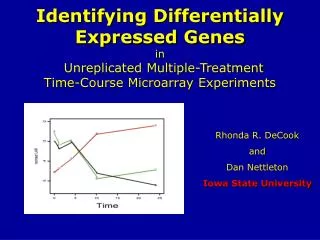
Identifying Differentially Expressed Genesin Unreplicated Multiple-TreatmentTime-Course Microarray Experiments Rhonda R. DeCook and Dan Nettleton Iowa State University
Experiment Background • J – treatments • K – time points for measurement collection • G - genes • One microarray for each treatment/time combination (giving J·K total microarrays) • Non-repeated measures. Different • experimental units for each time point • Post-normalized microarray data
An Example Experiment Hours of Exposure to UVA Radiation 0 1 4 24 10 Wild Type Genotype Mutant 1 Mutant 2
Genes of Interest • Treatment effects • Time effects • Interaction between • treatment and time • Any departure from coincident lines • with zero slope
Tests of Interest • We assume that where for any given g. • For every gene, we wish to test for all j,k against all alternatives. • The gthnull hypothesis says that the distribution • of gene expression for gene g is identical for all • combinations of treatment level and time point.
Identifying Genes of Interest • A cell-means model has 0 d.f. for error. • Instead we consider regression models with time as a quantitative variable (13 possible models). • Simplest models are linear in time or have only treatment effects. • The most complicated model has treatment effects and is cubic in time with all possible treatment x time interactions (3 d.f. for error).
Analysis 1. Use BIC to select the “best” model for each gene among the 13 alternative models considered. 2. Separately for each gene, compute a reduced-vs.-full model F-statistic with the “best” model as the full model. 3. Randomly assign the data vectors associated with each GeneChip to the combinations of treatment and time. 4. Recompute the same F-statistic computed in step 2 using the permuted data.
Analysis (ctd.) 5. Repeat steps 3 and 4 B times yielding for each gene g. 6. For each gene g, compute a p-statistic: Note that will tend to be smaller than a proper permutation p-value because the F-statistic used for gene gwas chosen using BIC to favor the alternative hypothesis.
Analysis (ctd.) 7. For each of the permuted data sets and each gene g, compute a p-statistic : a) Choose “best” model for each permuted data set and gene using BIC. b) Compute relevant F-statistic for all other data sets. c) Find the proportion of F-statistics from the other data sets that match or exceed the F-statistic for the permuted data set in question. 8. Compute a permutation p-value for each gene:
Histogram of P-Values Number of P-Values P-Value
Accounting for Many Tests • Many dependent hypothesis tests • Controlling the probability of even one type I error is too conservative • Use Storey and Tibshirani’s method to estimate a False Discovery Rate ‘Estimating the FDR under dependence, with applications to DNA microarrays’ (2001) • Compare observed p-value distribution • with the ‘average’ null distribution
Histogram of P-Values for the Observed Data Histogram of P-Values Averaged over 2499 Permuted Data Sets Number of P-Values Number of P-Values P-Value P-Value
Zooming in on Smallest P-Values Histogram of P-Values for the Observed Data Histogram of P-Values Averaged over 2499 Permuted Data Sets Number of P-Values Number of P-Values P-Value P-Value
Zooming in on Smallest P-Values Histogram of P-Values for the Observed Data Histogram of P-Values Averaged over 2499 Permuted Data Sets Ratio of bar heights is ~11% Number of P-Values Number of P-Values P-Value P-Value
Zooming in on Largest P-Values Histogram of P-Values for the Observed Data Histogram of P-Values Averaged over 2499 Permuted Data Sets Number of P-Values Number of P-Values P-Value P-Value
Zooming in on Largest P-Values Histogram of P-Values for the Observed Data Histogram of P-Values Averaged over 2499 Permuted Data Sets Ratio of bar heights is ~59% Number of P-Values Number of P-Values P-Value P-Value
Estimating the False Discovery Rate (FDR) 94 p-values computed from the observed data are less than or equal 0.002. The average number of p-values less than or equal to 0.002 in the 2499 permuted data sets is 10.273. An initial estimate of FDR is 10.273/94 10.9%
Estimating the False Discovery Rate (FDR) The initial estimate of 10.9% is too high because the estimate is based on assuming that all null hypotheses are true.
Estimating the False Discovery Rate (FDR) 488 p-values computed from the observed data are greater than or equal to 0.9. The average number of p-values greater than or equal to 0.9 in the 2499 permuted data sets is 827.699. Thus we estimate that 488/827.69959% of the null hypotheses are true in our data set.
Estimating the False Discovery Rate (FDR) Our final estimate of the FDR for p<=0.002 is
Estimating the False Discovery Rate (FDR) Our final estimate of the FDR for p<=0.002 is Estimated number of p-values<=0.002 if all null hypothesis were true Number of p-values >=0.9 Estimated number of p-values>=0.9 if all null hypotheses were true Number of p-values <=0.002
Key Points of Method • Partitions gene set according to best fitting model • Requires few assumptions about gene • expression distributions. • Has power to detect a variety of • alternatives to the null when replication • is lacking.
Acknowledgements Rhonda DeCook, Iowa State University Department of Statistics Carol Foster, Iowa State University Department of Botany Eve Wurtele, Iowa State University Department of Botany