Hydrologic Design Storms
Hydrologic Design Storms. Reading: Applied Hydrology Sections 14-1 to 14-4. Hydrologic design. Water control Peak flows, erosion, pollution, etc. Water management Domestic and industrial use, irrigation, instream flows, etc Tasks Determine design inflow Route the design inflow


Hydrologic Design Storms
E N D
Presentation Transcript
Hydrologic Design Storms Reading: Applied Hydrology Sections 14-1 to 14-4
Hydrologic design • Water control • Peak flows, erosion, pollution, etc. • Water management • Domestic and industrial use, irrigation, instream flows, etc • Tasks • Determine design inflow • Route the design inflow • Find the output • check if it is sufficient to meet the demands (for management) • Check if the outflow is at safe level (for control)
Return Period • Random variable: • Threshold level: • Extreme event occurs if: • Recurrence interval: • Return Period: Average recurrence interval between events equalling or exceeding a threshold • If p is the probability of occurrence of an extreme event, then or
More on return period • If p is probability of success, then (1-p) is the probability of failure • Find probability that (X ≥ xT) at least once in N years.
Risk Analysis • Uncertainty in hydrology • Inherent - stochastic nature of hydrologic phenomena • Model – approximations in equations • Parameter – estimation of coefficients in equations • Consideration of Risk • Structure may fail if event exceeds T–year design magnitude • R = P(event occurs at least once in n years) • Natural inherent risk of failure
Example 13.2.2 • Expected life of culvert = 10 yrs • Acceptable risk of 10 % for the culvert capacity • Find the design return period • What is the chance that the culvert designed for an event of 95 yr return period will have its capacity exceeded at least once in 50 yrs? The chance that the capacity will not be exceeded during the next 50 yrs is 1-0.41 = 0.59
Hydroeconomic Analysis • Probability distribution of hydrologic event and damage associated with its occurrence are known • As the design period increases, capital cost increases, but the cost associated with expected damages decreases. • In hydroeconomic analysis, find return period that has minimum total (capital + damage) cost.
Design Storms • Get Depth, Duration, Frequency Data for the required location • Select a return period • Convert Depth-Duration data to a design hyetograph.
TP 40 • Hershfield (1961) developed isohyetal maps of design rainfall and published in TP 40. • TP 40 – U. S. Weather Bureau technical paper no. 40. Also called precipitation frequency atlas maps or precipitation atlas of the United States. • 30mins to 24hr maps for T = 1 to 100 • Web resources for TP 40 and rainfall frequency maps • http://www.tucson.ars.ag.gov/agwa/rainfall_frequency.html • http://www.erh.noaa.gov/er/hq/Tp40s.htm • http://hdsc.nws.noaa.gov/hdsc/pfds/
2yr-60min precipitation map This map is from HYDRO 35 (another publication from NWS) which supersedes TP 40
An example of precipitation frequency estimates for a location in California 37.4349 N 120.6062 W
Design areal precipitation • Point precipitation estimates are extended to develop an average precipitation depth over an area • Depth-area-duration analysis • Prepare isohyetal maps from point precipitation for different durations • Determine area contained within each isohyet • Plot average precipitation depth vs. area for each duration
Depth-area curve (World Meteorological Organization, 1983)
Extreme Rainfalls, Station 1600 Values in inches for depth and inches per hour for intensity
Depth (intensity)-duration-frequency • DDF/IDF – graph of depth (intensity) versus duration for different frequencies • TP 40 or HYDRO 35 gives spatial distribution of rainfall depths for a given duration and frequency • DDF/IDF curve gives depths for different durations and frequencies at a particular location • TP 40 or HYDRO 35 can be used to develop DDF/IDF curves • Depth (P) = intensity (i) x duration (Td)
Example 14.2.1 • Determine i and P for a 20-min duration storm with 5-yr return period in Chicago From the IDF curve for Chicago, i = 3.5 in/hr for Td = 20 min and T = 5yr P = i x Td = 3.5 x 20/60 = 1.17 in
Equations for IDF curves IDF curves can also be expressed as equations to avoid reading from graphs i is precipitation intensity, Td is the duration, and c, e, f are coefficients that vary for locations and different return periods This equation includes return period (T) and has an extra coefficient (m)
Example 14.2.4 Using IDF curve equation, determine 10-yr 20-min design rainfall intensities for Denver From Table 14.2.3 in the text, c = 96.6, e = 0.97, and f = 13.9 Similarly, i = 4.158 and 2.357 in/hr for Td = 10 and 30 min, respectively
IDF curves for Austin Source: City of Austin, Watershed Management Division
Design Precipitation Hyetographs • Most often hydrologists are interested in precipitation hyetographs and not just the peak estimates. • Techniques for developing design precipitation hyetographs • SCS method • Triangular hyetograph method • Using IDF relationships (Alternating block method)
SCS Method • SCS (1973) adopted method similar to DDF to develop dimensionless rainfall temporal patterns called type curves for four different regions in the US. • SCS type curves are in the form of percentage mass (cumulative) curves based on 24-hr rainfall of the desired frequency. • If a single precipitation depth of desired frequency is known, the SCS type curve is rescaled (multiplied by the known number) to get the time distribution. • For durations less than 24 hr, the steepest part of the type curve for required duraction is used
Choice of Calibration Storms Representative? • In temporal shape 2007 Storm 2010 Hermine Storm
SCS Method Steps • Given Td and frequency/T, find the design hyetograph • Compute P/i (from DDF/IDF curves or equations) • Pick a SCS type curve based on the location • If Td = 24 hour, multiply (rescale) the type curve with P to get the design mass curve • If Td is less than 24 hr, pick the steepest part of the type curve for rescaling • Get the incremental precipitation from the rescaled mass curve to develop the design hyetograph
Example – SCS Method • Find - rainfall hyetograph for a 25-year, 24-hour duration SCS Type-III storm in Harris County using a one-hour time increment • a = 81, b = 7.7, c = 0.724 (from Tx-DOT hydraulic manual) • Find • Cumulative fraction - interpolate SCS table • Cumulative rainfall = product of cumulative fraction * total 24-hour rainfall (10.01 in) • Incremental rainfall = difference between current and preceding cumulative rainfall TxDOT hydraulic manual is available at: http://manuals.dot.state.tx.us/docs/colbridg/forms/hyd.pdf
SCS – Example (Cont.) If a hyetograph for less than 24 needs to be prepared, pick time intervals that include the steepest part of the type curve (to capture peak rainfall). For 3-hr pick 11 to 13, 6-hr pick 9 to 14 and so on.
ta tb Rainfall intensity, i h Td Time Triangular Hyetograph Method Td: hyetograph base length = precipitation duration ta:time before the peak r: storm advancement coefficient = ta/Td tb: recession time = Td – ta = (1-r)Td • Given Td and frequency/T, find the design hyetograph • Compute P/i (from DDF/IDF curves or equations) • Use above equations to get ta, tb, Td and h (r is available for various locations)
Triangular hyetograph - example • Find - rainfall hyetograph for a 25-year, 6-hour duration in Harris County. Use storm advancement coefficient of 0.5. • a = 81, b = 7.7, c = 0.724 (from Tx-DOT hydraulic manual) 3 hr 3 hr Rainfall intensity, in/hr 2.24 6 hr Time
Alternating block method • Given Td and T/frequency, develop a hyetograph in Dt increments • Using T, find i for Dt, 2Dt, 3Dt,…nDt using the IDF curve for the specified location • Using i compute P for Dt, 2Dt, 3Dt,…nDt. This gives cumulative P. • Compute incremental precipitation from cumulative P. • Pick the highest incremental precipitation (maximum block) and place it in the middle of the hyetograph. Pick the second highest block and place it to the right of the maximum block, pick the third highest block and place it to the left of the maximum block, pick the fourth highest block and place it to the right of the maximum block (after second block), and so on until the last block.
Example: Alternating Block Method Find: Design precipitation hyetograph for a 2-hour storm (in 10 minute increments) in Denver with a 10-year return period 10-minute