Understanding Approximations in Probability Distributions
Learn how to approximate binomial and Poisson distributions using normal distribution. Explore scenarios and calculations with examples on exponential and uniform distributions.


Understanding Approximations in Probability Distributions
E N D
Presentation Transcript
More on Continuous Probability Distributions QSCI 381 – Lecture 20
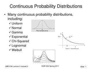
Approximating a Binomial Distribution-I • It is possible to compute approximate probabilities for the binomial distribution using the normal distribution. • If np 5 and nq 5, the binomial random variable X ~B(n,p) is approximately normally distributed: • This approximation can be quite accurate even though the binomial distribution is discrete and the normal distribution is continuous.
Approximating a Binomial Distribution-II • We need an interval when defining the probability associated with a discrete value for x using the normal distribution, i.e. PB(X=x) is approximated byPN(x-Δ<X<x+Δ). • We call Δ the correction for continuity and set it to 0.5.
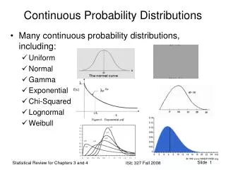
Approximating a Binomial Distribution-III n=30 p=0.25
Approximating a Binomial Distribution-IV(Guidelines) • Specify the values for n, p, and q. • Can the normal distribution be used for approximation purposes, i.e. is np5, nq5? • Find the mean and standard deviation for the approximating normal distribution. • Apply the continuity correction. • Find the approximate z-score and calculate the probability.
Approximating a Binomial Distribution • 175 salmon enter a stream. If the probability of reaching the spawning ground is 0.3, what is the probability that less than 50 reach the spawning grounds? • n=175; p=0.3; np=52.5; nq=122.5. • =52.5; =6.06 • x = 49.5 so z = (49.5-52.5)/6.06=-0.495 • Using NORMDIST, this value of z corresponds to P=0.31
Approximating a Poisson Distribution • It is possible to compute approximate probabilities for the Poisson distribution using the normal distribution. • If >10, the Poisson random variable X ~P() is approximately normally distributed:
Approximating a Poisson Distribution(Example-I) • Suppose the average number of salmon passing a counting weir is 5 per minute. What is the probability that in a 15 minute period more than 85 salmon pass the weir?
Approximating a Poisson Distribution(Example-II) • We first need to express the mean rate in terms of numbers per 15 minute interval, =15*5=75. • >10 so we can use the normal approximation. • The z-score = (85.5-75)/75=1.212. This corresponds to a probability of 0.887 of 85 or less salmon passing in 15 minutes or 0.113 of more than 85 salmon passing in 15 minutes. Note: 85 is replaced by 85.5 because we need the probability of 85 or fewer animals.
The Exponential Distribution-I • The Poisson distribution arose when counting the number of events in an interval. The exponential distribution considers the interval of time between events. • If events are occurring at random with average rate of per interval, then the probability density function for the length of time between events is:
The Exponential Distribution-II(Example-I) • If a herring spawns 1.5 times per week on average, what is the probability that it doesn’t spawn for 2 weeks? • Note that this is a continuous probability distribution so we are looking for the area under the curve: (wks)
The Exponential Distribution-II(Example-II) • Solution: • P[X>2] = 1-P[X2]=0.0498 • I used the EXCEL function: • EXPONDIST(x,,cum)
The Uniform Distribution • This is the simplest possible continuous distribution. It is used to deal with the situation where all values in some interval (a, b) are equally likely. • Notation: • The probability density function for the uniform distribution is:
The Uniform Distribution(Example) • Suppose the mass of a nominally 500 kg bag of fish is equally likely to lie between 480 and 505 kg. What is the probability that the bag contains at least the advertised mass of fish?