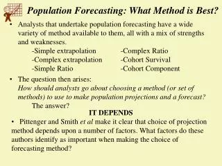
Population Forecasting
Population Forecasting. Time Series Forecasting Techniques. Wayne Foss, MBA, MAI Wayne Foss Appraisals, Inc . Email: wfoss@fossconsult.com. Extrapolation Techniques. Real Estate Analysts - faced with a difficult task long-term projections for small areas such as Counties Cities and/or

Population Forecasting
E N D
Presentation Transcript
Population Forecasting Time Series Forecasting Techniques Wayne Foss, MBA, MAI Wayne Foss Appraisals, Inc. Email: wfoss@fossconsult.com
Extrapolation Techniques • Real Estate Analysts - faced with a difficult task • long-term projections for small areas such as • Counties • Cities and/or • Neighborhoods • Reliable short-term projections for small areas • Reliable long-term projections for regions countries • Forecasting task complicated by: • Reliable, Timely and Consistent information
Sources of Forecasts • Public and Private Sector Forecasts • Public: California Department of Finance • Private: CACI • Forecasts may be based on large quantities of current and historical data
Projections are Important • Comprehensive plans for the future • Community General Plans for • Residential Land Uses • Commercial Land Uses • Related Land Uses • Transportation Systems • Sewage Systems • Schools
Definitions • Estimate: • “is an indirect measure of a present or past condition that can be directly measured.” • Projection (or Prediction): • “are calculations of future conditions that would exist as a result of adopting a set of underlying assumptions.” • Forecast: • “is a judgmental statement of what the analyst believes to be the most likely future.”
Projections vs. Forecasts • The distinction between projections and forecasts are important because: • Analysts often use projections when they should be using forecasts. • Projections are mislabeled as forecasts • Analysts prepare projections that they know will be accepted as forecasts without evaluating the assumptions implicit in their analytic results.
Procedure • Using Aggregate data from the past to project the future. • Data Aggregated in two ways: • total populations or employment without identifying the subcomponents of local populations or the economy • I.e.: age or occupational makeup • deals only with aggregate trends from the past without attempting to account for the underlying demographic and economic processes that caused the trends. • Less appealing than the cohort-component techniques or economic analysis techniques that consider the underlying components of change.
Why Use Aggregate Data? • Easier to obtain and analyze • Conserves time and costs • Disaggregated population or employment data often is unavailable for small areas
Extrapolation: A Two Stage Process • Curve Fitting - • Analyzes past data to identify overall trends of growth or decline • Curve Extrapolation - • Extends the identified trend to project the future
Assumptions and Conventions • Graphic conventions Assume: • Independent variable: x axis • Dependent variable: y axis • This suggests that population change (y axis) is dependent on (caused by) the passage of time! • Is this true or false?
Assumptions and Conventions • Population change reflects the change in aggregate of three factors: • births • deaths • migration • These factors are time related and are caused by other time related factors: • health levels • economic conditions • Time is a proxy that reflects the net effect of a large number of unmeasured events.
Caveats • The extrapolation technique should never be used to blindly assume that past trends of growth or decline will continue into the future. • Past trends observed, not because they will always continue, but because they generally provide the best available information about the future. • Must carefully analyze: • Determine whether past trends can be expected to continue, or • If continuation seems unlikely, alternatives must be considered
Alternative Extrapolation Curves • Linear • Geometric • Parabolic • Modified Exponential • Gompertz • Logistic
Linear Curve • Formula: Yc = a + bx • a = constant or intercept • b = slope • Substituting values of x yields Yc • Conventions of the formula: • curve increases without limit if the b value > 0 • curve is flat if the b value = 0 • curve decreases without limit if the b value < 0
Geometric Curve • Formula: Yc = abx • a = constant (intercept) • b = 1 plus growth rate (slope) • Difference between linear and geometric curves: • Linear: constant incremental growth • Geometric: constant growth rate • Conventions of the formula: • if b value > 1 curve increases without limit • b value = 1, then the curve is equal to a • if b value < 1 curve approaches 0 as x increases
Parabolic Curve • Formula: Yc = a + bx + cx2 • a = constant (intercept) • b = equal to the slope • c = when positive: curve is concave upward when = 0, curve is linear when negative, curve is concave downward growth increments increase or decrease as the x variable increases • Caution should be exercised when using for long range projections. • Assumes growth or decline has no limits
Modified Exponential Curve • Formula: Yc = c + abx • c = Upper limit • b = ratio of successive growth • a = constant • This curve recognizes that growth will approach a limit • Most municipal areas have defined areas • i.e.: boundaries of cities or counties
Gompertz Curve • Formula: Log Yc = log c + log a(bx) • c = Upper limit • b = ratio of successive growth • a = constant • Very similar to the Modified Exponential Curve • Curve describes: • initially quite slow growth • increases for a period, then • growth tapers off • very similar to neighborhood and/or city growth patterns over the long term
Logistic Curve • Formula: Yc = 1 / Yc-1 where Yc-1 = c + abX • c = Upper limit • b = ratio of successive growth • a = constant • Identical to the Modified Exponential and Gompertz curves, except: • observed values of the modified exponential curve and the logarithms of observed values of the Gompertz curve are replaced by the reciprocals of the observed values. • Result: the ratio of successive growth increments of the reciprocals of the Yc values are equal to a constant • Appeal: Same as the Gompertz Curve
Selecting Appropriate Extrapolation Projections • First: Plot the Data • What does the trend look like? • Does it take the shape of any of the six curves • Curve Assumptions • Linear: if growth increments - or the first differences for the observation data are approximately equal - • Geometric: growth increments are equal to a constant
Selecting Appropriate Extrapolation Projections, con’t • Curve Assumptions • Parabolic: Characterized by constant 2nd differences (differences between the first difference and the dependent variable) if the 2nd differences are approximately equal • Modified Exponential: characterized by first differences that decline or increase by a constant percentage; ratios of successive first differences are approximately equal
Selecting Appropriate Extrapolation Projections, con’t • Curve Assumptions • Gompertz: Characterized by first differences in the logarithms of the dependent variable that decline by a constant percentage • Logistic: characterized by first differences in the reciprocals of the observation value that decline by a constant percentage • Observation data rarely correspond to any assumption underlying the extrapolation curves
Selecting Appropriate Extrapolation Projections, con’t • Test Results using measures of dispersion • CRV (Coefficient of relative variation) • ME (Mean Error) • MAPE (Mean Absolute Percentage Error) • In General: Curve with the lowest CRV,ME and MAPE should be considered the best fit for the observation data • Judgement is required • Select the Curve that produces results consistent with the most likely future
Housing Unit Method • Formulas: • 1) HHg = ((BP*N)-D+HUa)*OCC • 2) POPg = HHg * PHH • 3) POPf = POPc + POPg • Where: HHg Growth In Number of Households • BP Average Number of Bldg. Permits issued per year since most recent census • N Forecast period in Years • HUa No. of Housing Units in Annexed Area • OCC Occupancy Rate • POPg Population Growth • PHH Persons per Household • POPc Population at last census • POPf Population Forecast
Housing Unit Method Example • Forecast Growth in Number of Housing Units • 1) HHg = ((BP*N)-D+HUa)*OCC • HHg = ((193*5)-0+0)*95.1% • HHg = 918 • Forecast Growth in Population • 2) POPg = HHg * PHH • POPg = 918 * 2.74 • POPg = 2,515 • Forecast Total Population • 3) POPf = POPc + POPg • POPf = 126,003 + 2,515 • POPf = 128,518
So That’s Population Forecasting Are there any Questions? Wayne Foss, MBA, MAI, Fullerton, CA USA Email: waynefoss@usa.net

