Sub-Nyquist Radar Sensing
Sub-Nyquist Radar Sensing. Gal Itzhak , Eliahu Baransky Supervised by Noam Wagner, Idan Shmuel and Prof. Yonina C. Eldar. Agenda. Introduction – Describing the problem Finite Rate of Innovation High-Level System Architecture Parametric Estimation Algorithms Testing & Simulations

Sub-Nyquist Radar Sensing
E N D
Presentation Transcript
Sub-Nyquist Radar Sensing Gal Itzhak, EliahuBaransky Supervised by Noam Wagner, IdanShmuel and Prof. Yonina C. Eldar
Agenda • Introduction – Describing the problem • Finite Rate of Innovation • High-Level System Architecture • Parametric Estimation Algorithms • Testing & Simulations • Hardware Implementation • Comparison with Classical Approaches • Future Goals • References
Introduction • A radar is an object detection device that operates on short RF pulses. • A pulse of known shape is sent to a specific direction, and its reflection from target objects are detected at the radar. • The arrival time (or delay) of a reflection directly relates to the target’s distance by the formula • The fundamental problem of radars is to give an estimate of the arrival time, despite noise and distortions corrupting the signal. • Some basic properties of a radar are: • PRI – Pulse Repetition Interval • PRF – Pulse Repetition Frequency – 1/PRI • Temporal Resolution – 1/BW • Maximal Detection Range -
Mathematical Model • A simplistic model of the radar problem is given by the following equation, examined over a single PRI: Where are the unknown gains and delays of each path, is the pulse, and is an additive white Gaussian noise. • Our goal is to retrieve the amplitudes and the time delays in the highest possible precision.
Classical Sampling • Classical estimation algorithms (e.g. matched-filtering) require us to sample the radar signal at its Nyquist rate. • Since higher bandwidths result in higher detection resolution, as the demand for resolution increases, so does the required sampling rate. • As an example, 2[ns] pulses require approximately 1[GHz] sampling rate. Such high rates require fast hardware, large power consumption and result in a lot of redundant data that needs to be stored in hardware memory.
Finite Rate of Innovation • Since our pulse shape is known, there are only unknowns per PRI (Finite Rate of Innovation – FRI). • With generalized sampling methods, ideally we need only samples per PRI to recover precisely the unknowns. • As an example, for pulses, the rate at the analog-to-digital converters can be theoretically reduced to instead of
Finite Rate of Innovation • Reducing the sampling rate to the theoretical bound is achievable only through ideal hardware and in noise-free environments. • To devise schemes that are both implementable in real hardware and that are robust noise, we examine (1) in the frequency-domain • Acquiring samples of the signal spectrum, allows us to construct a system equation that can be solved through various techniques.
High-Level System Architecture • Two-Phase Reconstruction • The first stage is analog compression using standard analog devices (filters, splitters, ADC’s, etc.) • The second stage is digital recovery algorithm, which may be implemented on FPGA. • In order to understand the first stage, we begin by examining the second stage. Signal Generator Low-Rate ADC AWR Model FPGA Analog Pre Processing
Parametric Estimation Algorithms • In all further discussion we restrict ourselves to discrete frequencies, integer multiples of 1KHz (the best we can achieve with interval) • To estimate the unknowns, we shall acquire samples of the spectrums in arbitrary frequency constellations.
Spectral Estimation • We can re-formulate the problem in (2) as sum of exponentials problem, where plays the role of time, and play the role of the unknown frequencies. • There are many known mature techniques to solve these kind of problems. These techniques require the sampling to be uniformly spaced, and therefore force us to use consecutive sets of samples. • We have focused on the Matrix Pencil algorithm.
Matrix Pencil • Use the observations to form the matrix Where is a user parameter. • Carry out a SVD decomposition to obtain • Perform thresholding on the singular values in the matrix . Take only values so that The number of unfiltered singular values corresponds to the number of exponentials (pulses) in the signal. Filter the columns of V according to the filtering of the singular values, and obtain the matrix V’. • Obtain V1’ by removing the last row from V’. Obtain V2’ by removing the first row from V’. Find the eigenvalues of the matrix • Obtain the delay estimation from the eigenvalues:
Compressed Sensing • Another point of view on (2) is a sparse linear combination of a known basis. As this basis is infinite, we quantize the time grid: where is a set of pre-determined Fourier coefficients. • Formulating a matrix with as its columns, we can approximate (2) by: assuming that is a L-sparse vector. • We use the OMP Algorithm to retain the sparse vector .
Orthogonal Matching Pursuit • Initialize • While stopping criteria not met 1. Obtain the projections, 2. Set 3. Orthogonalize selected vector with respect to previous selections , 4. Augment the matrix with as a column 5. Obtain the residual, 6. Increment counter, • The stopping criteria can be either residual energy , or pre-determined pulse number .
Simulation Setup • To achieve noise robustness, an oversampling factor is introduced: • The variance of the noise, as a function of the SNR, was defined as • Both algorithms were tested under many different parametric conditions.
Performance Measures • We have employed two metrics to measure the performance of the algorithms: • The permutation was selected to maximize the hit rate. • These metrics were averaged over a high number of scenarios.
Simulation Results • Comparing Matrix Pencil and different OMP constellations:
Simulation Results • In order to find an optimal OMP constellation, and optimize the resolution of the sensing dictionary, we have used the result • Hardware constraints (see further slides) forced us to select the samples from four frequency-bands, each wide and distributed arbitrarily over the pulse spectra. • Parallelizing the computation, we have tested nearly 500 different constellations, each probed with 500 different scenarios, so that we can achieve a correct statistical result. • All later simulations were performed with assumed SNR of
Optimal Constellations • From the results, we have selected two constellations that provided the best results • One in the range , with exterior bands . • One in the range , with exterior bands . • In these ranges, we have performed another search, trying to find yet a better constellation, while fixing the exterior bands.
Hardware Implementation • [1],[2] and [3] suggest several sampling schemes that achieve the minimal theoretical sampling rate. Two of these are: • Both schemes required narrow-band filters with large Q-factors, or idealistic oscillators, that are not available in current technology. Multi-Channel Integrators Sum-of-Sincs Filtering
Hardware Implementation • Given these limitations, we were forced to select grouped constellations. • In order to sample them we use band-pass filters and modulators, as shown in next slides.
Hardware Implementation BPF 600-660Khz LPF 4 Ch. A2D Splitter 1->4 LPF 1.7Mhz BPF 1200-1270Khz LPF BPF 1430-1490Khz LPF BPF 1580-1640Khz LPF Sin(1500Khz)
Hardware Implementation Sin(8Mhz) BPF 260-310Khz LPF 4 Ch. A2D Splitter 1->4 BPF 8.1-10.3Mhz BPF 1.2-1.3Mhz LPF BPF 1.4-1.5Mhz LPF BPF 2.1-2.2Mhz LPF Sin(2Mhz)
Comparison to Matched Filtering • Matched Filtering is an algorithm that locates the discrete time at which the sampled signal has maximal correlation with the pulse shape. • It requires fast sampling (more than Nyquist) • Testing the method with our pulse model, with sample noise, we have achieved the following results: • With sampling rate, the hit rate was 45.7% and an estimation error of 49[ns] • Our scheme supports (and less) sampling rate at four channels, while achieving results comparable to those of matched filtering with sampling rate. A 10,000x improvement.
Other Solutions • Spectral estimation can be performed by various techniques, such as: MUSIC, ESPRIT, Cadzow denoising, annihilating filter and more. • In the compressed sensing frame, sparse reconstruction is performed by: thresholding, basis pursuit, SPICE, LIKES and others.
Future Goals • To optimize performance, our goals now are to research and develop algorithms that use the basic idea of the OMP but further increase hit rate and decrease resolution. • Once these algorithms were devised, we will test them with different conditions and parameters, to achieve optimal performance, and to compare them to OMP.
References [1] Ronen Tur, Y.C. Eldar and Zvi Friedman, “Innovation Rate Sampling of Pulse Streams With Application to Ultrasound Imaging”, IEEE Trans. Signal Process., vol. 59, no. 4, pp. 1827-1842, 2011 [2] K. Gedalyahu, R. Tur and Y.C. Eldar, “Multichannel Sampling of Pulse Streams at the Rate of Innovation”, IEEE Trans. Signal Process., vol. 59, no. 4, pp. 1491-1504, 2011 [3] K. Gedalyahu and Y. C. Eldar, "Time-delay estimation from low-rate samples: A union of subspaces approach", IEEE Trans. Signal Process., vol. 58, no. 6, pp. 3017-3031, 2010 [4] T. K. Sarkar and Odilon Pereira, “Using the Matrix Pencil Method to Estimate the Parameters of a Sum of Complex Exponentials”, IEEE Antennas and Propagation Magazine, vol. 37, no. 1, pp. 48-55, 1995 [5] M. Gharavi-Alkhansariand T. S. Huang, “A fast orthogonal matching pursuit algorithm”, Acoustics, Speech and Signal processing, proceedings of the 1998 IEEE international conference, Seattle, WA, pp. 1389-1392 vol.3, 1998. [6] P. Stoica and P. Babu, “Sparse Estimation of Spectral Lines: Grid Selection Problems and Their Solutions”, IEEE Trans. Signal Process., vol. 60, no. 2, pp. 962-967, 2012 [7] George L. Turin, “An Introduction to Matched Filters”, IRE Trans. Information Theory, vol. 6, no. 3, pp. 311-329, 1960