Fault Detection by a Seismic Scanning Tunneling Macroscope
280 likes | 455 Vues
Fault Detection by a Seismic Scanning Tunneling Macroscope. Sherif M. Hanafy. Outline. Introduction Motivation. Get super resolution by TRM Method. TRM & mute-window test Synthetic Test. 2D elastic simulation Field Test. 3D fault test Conclusions. Outline.

Fault Detection by a Seismic Scanning Tunneling Macroscope
E N D
Presentation Transcript
Fault Detection by a Seismic Scanning Tunneling Macroscope Sherif M. Hanafy
Outline • Introduction • Motivation. Get super resolution by TRM • Method. TRM & mute-window test • Synthetic Test. 2D elastic simulation • Field Test. 3D fault test • Conclusions
Outline • Introduction • Motivation. Get super resolution by TRM • Method. TRM & The mute-window test • Synthetic Test. 2D elastic simulation • Field Test. 3D fault test • Conclusions
Introduction: Resolution L X Z Depth Rayleigh resolution Δx Abbe resolution Super resolution
Outline • Introduction • Motivation. Get super resolution by TRM • Method. TRM & The mute-window test • Synthetic Test. 2D elastic simulation • Field Test. 3D fault test • Conclusions
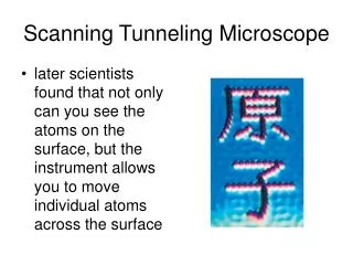
Motivation Motivation: Achieve super resolution IBM, 1986, Scanning Tunneling Microscope Problem:Source and receiver need to be in the near-field Solution:Use scatterer points
Outline • Introduction • Motivation. Get super resolution by TRM • Method. TRM & The mute-window test • Synthetic Test. 2D elastic simulation • Field Test. 3D fault test • Conclusions
Post-stack Migration Image Plane ZO Migration Formula Calculated Data Measured Data
Post-stack Migration with Point Scatterer Image Plane Measured Data Calculated Data ZO Migration Formula
Post-stack Migration with Point Scatterer |s-s0| ~ l/40 |s-s0| ~ l 0.2 0.7 0.2 0.7 S’ S’ Near-field->super-resolution Far-field->Rayleigh resolution
Time Reversal Mirrors (TRM) Image Plane ZO Migration Formula Calculated Data Measured Data
Time Reversal Mirrors (TRM) TRM Profile Image Plane ZO Migration Formula Calculated Data Measured Data Measured Data
Summary Image Plane |s-s0| ~ l/40 |s-s0| ~ l TRM Profile 0.2 0.7 0.2 0.7 S’ S’ Near-field->super-resolution Far-field->Rayleigh resolution
Outline • Introduction • Motivation. Get super resolution by TRM • Method. The mute-window test • Synthetic Test. 2D elastic simulation • Field Test. 3D fault test • Conclusions
Velocity Model 0 120 receivers at 1 m receiver interval 120 shots at 1 m shot interval Depth (m) 40 0 120 X (m) 500 3500 Vp (m/s) 250 1750 Vs (m/s) 2.0 2.6 Density (gm/cc)
TRM Profiles Source # 34 Source # 80 1 TRM Profile No traces are muted Amplitude 1 TRM Profile No traces are muted Amplitude -0.2 120 1 Trial Source -0.2 120 1 1 Trial Source TRM Profile 21 traces are muted Amplitude 1 TRM Profile 21 traces are muted Amplitude -0.2 120 1 Trial Source 1 TRM Profile 101 traces are muted -0.2 Amplitude 120 1 Trial Source 1 TRM Profile 101 traces are muted Amplitude -0.2 120 1 Trial Source -0.2 120 1 Trial Source
TRM Images Source # 34 Source # 80 a) TRM Image of Shot # 34 b) TRM Image of Shot # 80 0 0 Source Location Source Location Mute-window Size Mute-window Size 111 111 1 120 1 120 Trial Source Trial Source Scatterers in the near-field of the source Receiver are only at far-field Scatterers in the far-field of the source Receiver are only at far-field
Outline • Introduction • Motivation. Get super resolution by TRM • Method. TRM & The mute-window test • Synthetic Test. 2D elastic simulation • Field Test. 3D fault test • Summary
Field Test • Data Collected at Washington Fault Area, north of Arizona, USA. • 6 Lines of receivers/shots • 80 receivers/line at 1 m receiver interval • 40 shots/line at 2 m shot interval
Super Resolution Test Fault Pixel size: 2 x 1.5 m2 Wavelength: 10 m
Super Resolution Results Fault Migration Image – Traces within 0.8 λ are muted Migration Image – Traces within 0.4 λ are muted Migration Image – Traces within 0.1 λ are muted Migration Image using All Traces
Outline • Introduction • Motivation. Get super resolution by TRM • Method. TRM & The mute-window test • Synthetic Test. 2D elastic simulation • Field Test. 3D fault test • Conclusions
Conclusions • TRM profiles have the shape of a sink curve if no scatterer in the near-field of the shot point • TRM profiles have the shape of a spike if scatterer exists in the near-field of the shot point • Muting the near-field traces tends to decrease the amplitude of the TRM profile and its resolution |s-s0| ~ l/40 |s-s0| ~ l 0.2 0.7 0.2 0.7 S’ S’
Possible Applications Find local anomalies, faults, and scatterer points around boreholes in VSP data Ground Borehole