

SlideServe
Menu
Préférences
© SlideServe · v2026

PAVLOVIAN PARADIGM

watson avatar
21 diapositives · 387 Views · Aug 22, 2014

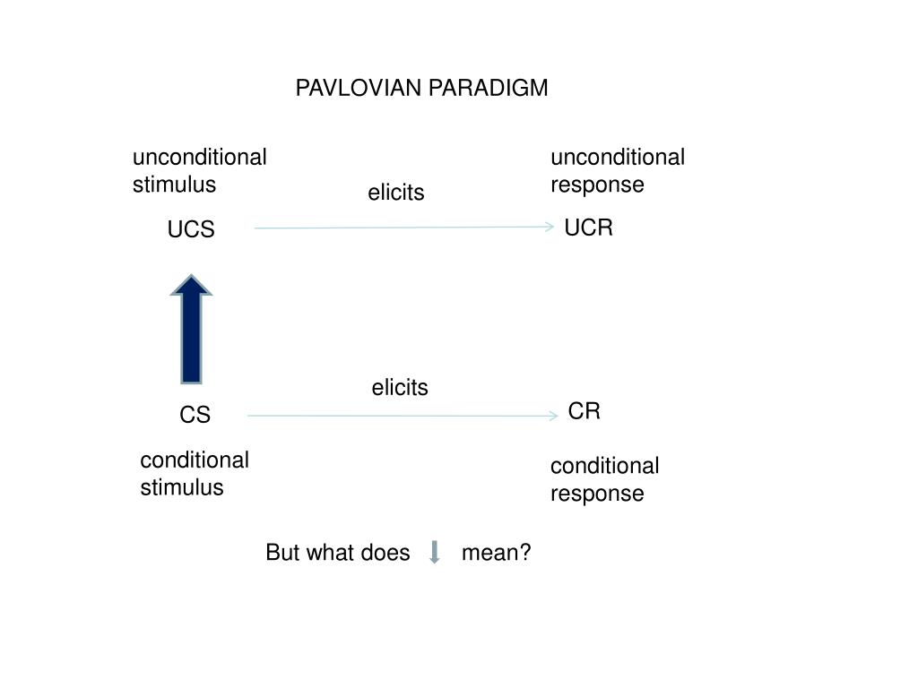
PAVLOVIAN PARADIGM. unconditional stimulus. unconditional response. elicits. UCR. UCS. elicits. CR. CS. conditional stimulus. conditional response. But what does mean?. Respondent Contingencies Standard Procedure P(UCS | CS) = 1 ; P(UCS |~ C S) = 0
PAVLOVIAN PARADIGM - slide 1
01 / 21PAVLOVIAN PARADIGM
1 / 17

Télécharger la présentation

PAVLOVIAN PARADIGM
Une image / un lien ci-dessous est fourni (tel quel) pour télécharger la présentation

Politique de téléchargement : le contenu du site vous est fourni TEL QUEL pour votre information et votre usage personnel ; il ne peut être vendu, concédé sous licence ni partagé sur d’autres sites sans l’accord de son auteur.Le contenu vous est fourni TEL QUEL, pour votre information et votre usage personnel uniquement. Téléchargez la présentation en cliquant sur ce lien. Lors du téléchargement, si vous ne parvenez pas à télécharger une présentation, l’éditeur a peut-être supprimé le fichier de son serveur.Pendant le téléchargement, si vous ne parvenez pas à obtenir une présentation, le fichier a peut-être été supprimé par l’éditeur.

F I N

Plus de contenu associé

Transcription de la présentation
  1. PAVLOVIAN PARADIGM unconditional stimulus unconditional response elicits UCR UCS elicits CR CS conditional stimulus conditional response But what does mean?

  2. Respondent Contingencies • Standard Procedure • P(UCS|CS) = 1 ; P(UCS|~CS) = 0 • Partial Reinforcement • 0 < P(UCS|CS) < 1 ; P(UCS|~CS) = 0 • Random Control • 0 < P(UCS|CS) = P(UCS|~CS) • Inhibitory CS • 0 < P(UCS|CS) < P(UCS|~CS) Pavlovian Conditioning

  3. Contingency Table UCS ~UCS #UCSCS = A # CS = A + B P(UCS|CS) = A / (A+B) CS B A+B A ~CS D C+D C A+C B+D N |AD - BC| (A+B)(C+D)(A+C)(B+D)  = Pavlovian Conditioning

  4. Staddon’s Data Pavlovian Conditioning

  5. Contingencies and Staddon’s Data SH ~SH = 20/30 = 2/3 = 10/30 = 1/3 = 10/30 = 1/3 = 20/30 = 2/3 P(S) P(~S) P(SH) P(~SH) 10 20 S 10 012 011 10 ~S 10 0 022 021 30 10 20 Pavlovian Conditioning

  6. Contingencies and Staddon’s Data If S and SH were independent (“random control”): P (SH|S) = P (SH) or P (SH  S) = P (SH) P(S) By definition: P (SH|S) = P (SH  S) = #(SH and S) P(S) #S = 10/20 = 1/2 But: P (SH) = 10/30 = 1/3 So: P (SH|S) ≠ P (SH). Also, P (SH  S) ≠ P (SH) P(S) 10/30 = 1/3 ≠ (1/3)(2/3) = 2/9 Pavlovian Conditioning

  7. = X²1df= │011022 – 012021│ • N (011 + 012)(021 + 022)(011 + 021)(012 +022) Recall X² test for independence in contingency table with observed frequencies 0ij rc i=1 j=1  Where the Eij’s are the Expected Frequencies X²1df = (0ij – Eij) ² Eij  For a 2 x 2 Table X²1df = N │011022 – 012021│² (011 + 012)(021 + 022)(011 + 021)(012 +022) Pavlovian Conditioning

  8. For a 2 x 2 Table Χ²1df = N │011022 – 012021│² (011 + 012)(021 + 022)(011 + 021)(012 +022) SH ~SH E11 = (011 + 012)(011 + 021) N E12 = (011 + 012)(012 + 022) N E21 = (021 + 022)(011 + 021) N E22 = (021 + 022)(012 + 022) N S 011 + 012 012 011 021 022 021 + 022 ~S N 012 + 022 011 + 021 Pavlovian Conditioning

  9. X1² = (13.33 – 10)² + (10 - 6.67)² 13.33 6.67 + (10 – 6.67)² + (3.33 -0)² 6.67 3.33 = 7.486 ≈ 7.5 X².95 = 3.84 1df  = │(10(0) – (10)(10) │= 100 = 0.5 (20)(10)(20)(10) (20)(10) ² = 0.25 = X1² / 30, so X1² = 7.5 as above. S and Shock are not independent • For Staddon’s Data, the table is: 011 = 10 E11 = 13.33 012 = 10 E12 = 6.67 20 022 = 0 E22 = 3.33 021 = 10 E21 = 6.67 10 30 10 20 Pavlovian Conditioning

  10. cs S = Rcs Rcs+ Rcs cs cs S = 0.0 S = 0.5 Pavlovian Conditioning

  11. P(UCS|CS) = P(UCS|~CS) = P(UCS~CS) = # (UCS~CS) P(~CS) # ~CS [P(CS) > 0] ~CS E UCSCS UCS~CS ~CS = E – CS = Context P(UCS|CS) = 1- P(~UCS|CS) P(UCS|~CS) = 1- P(~UCS|~CS) ~UCS Pavlovian Conditioning

  12. RESCORLA-WAGNER MODEL

  13. What are some characteristics of a good model? Variables well-described and manipulatable. Accounts for known results and able to predict non-trivial results of new experiments. Dependent variable(s) predicted in at least relative magnitude and direction. Parsimonious (i.e., minimum assumptions for maximum effectiveness).

  14. STEPS IN MODEL BUILDING • IDENTIFICATION: WHAT’S THE QUESTION? • ASSUMPTIONS: WHAT’S IMPORTANT; WHAT’S NOT? • CONSTRUCTION: MATHEMATICAL FORMULATION • ANALYSIS: SOLUTIONS • INTERPRETATION: WHAT DOES IT MEAN? • VALIDATION: DOES IT ACCORD WITH KNOWN DATA? • IMPLEMENTATION: CAN IT PREDICT NEW DATA?

  15. PRINCIPAL THEORETICAL VARIABLE: ASSOCIATIVE STRENGTH, V

  16. RESCORLA-WAGNER MODEL

  17. ASSUMPTIONS 1. When a CS is presented its associative strength, Vcs, may increase (CS+), decrease (CS-), or remain unchanged. 2. The asymptotic strength () of association depends on the magnitude (I) of the UCS:  = f (UCSI). 3. A given UCS can support only a certain level of associative strength, . 4. In a stimulus compound, the total associative strength is the algebraic sum of the associative strength of the components. [ex. T: tone, L: light. VT+L =VT + VL] 5. The change in associative strength, V, on any trial is proportional to the difference between the present associative strength, Vcs, and the asymptotic associative strength, .

  18. R-W Accounts for the Following • Acquisition • Extinction • Overshadowing • Blocking • Conditional Inhibition • and more.

  19. Contiguity in R-W Model If P(UCS|CS) = P(UCS|~CS), we really have CS = CS + CTX and ~CS = CTX. Then: P(UCS|CS + CTX) = P(UCS|CTX) V (CS + CTX) = VCS + VCTX (R-W axiom) V CS = V (CS +CTX) = VCS + VCTX but: V CTX = V ~CS so: V (CS + CTX) = V CS + V~CS = 0  No significant conditioning occurs to the CS Pavlovian Conditioning