Satellite remote sensing applications in Meteorology
1.54k likes | 2.63k Vues
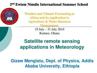
2 nd E wiem Nimdie International Summer School. Satellite remote sensing applications in Meteorology. Weather and Climate Forecasting in Africa and its Application to Agriculture & Water Resource Management. 19 July – 31 July 2010 Kumasi , Ghana.

Satellite remote sensing applications in Meteorology
E N D
Presentation Transcript
2ndEwiem Nimdie International Summer School Satellite remote sensing applications in Meteorology Weather and Climate Forecasting in Africa and its Application to Agriculture & Water Resource Management. 19 July – 31 July 2010 Kumasi, Ghana GizawMengistu, Dept. of Physics, Addis Ababa University, Ethiopia
Outline 1. Introduction • Meteorological satellites • Instrumentation 2. Retrieval of meteorological parameters • Measurement of sea and land surface temperature • Retrieval of vertical profiles of temperature and humidity 3. Measurement of rainfall • Visible & Infra-red (IR)
Outline 4. Measurement of winds • Cloud motion vectors (CMV) 5. Satellite image/signal • Satellite image/signal interpretation
1. Introduction • Meteorological satellites • Satellites instrumentation
First application of satellite remote sensing • Began with TIROS1, launched in April 1960 • Simple TV system on board to map clouds • Satellites are now a vital an integral part of our weather forecasting system.
Satellite remote sensing • Now both polar orbiting and geostationary satellites are used • Polar orbiters operate in a similar way to other remote sensing satellites (Landsat, SPOT etc.) • Geostationary satellites continually view the same portion of the Earth.
Satellite remote sensing Geostationary Satellites • Orbit above the equator at 35,800 Km and complete one orbit every 24hrs. • Remain over the same point on the surface of the Earth. • Continually view the same portion of the Earth. • A network provides coverage of the entire globe
Satellite remote sensing Major Applications • Solar radiation exposure • Uses a model based on an advanced estimate of cloud cover • Cloud and Water Vapour Motion vectors • Tracks identifiable cloud features • Entered into weather forecasting models
Instrument Observing Characteristics Observations depend on • telescope characteristics (resolving power, diffraction) • detector characteristics (signal to noise) • communications bandwidth (bit depth) • spectral intervals (window, absorption band) • time of day (daylight visible) • atmospheric state (T, Q, clouds) • earth surface (Ts, vegetation cover)
2. Retrieval of meteorological parameters • Measurement of sea and land surface temperature; • Retrieval of vertical profiles of temperature and humidity.
Definition Radiance is the amount of energy/per unit time/per area of a detector/per spectral interval/per solid angle
Surface Temperature and Emissivity Estimation The radiance at the sensor is given by LS j =[εjLjBB(T)+(1-εj)Ljsky]*t+Ljatm Where εj is surface emissivity , LjBB is spectral radiance of a blackbody at the surface at temperature T, Ljsky is spectral radiance incident upon the surface from the Atmosphere, calculated using radiative transfer equation (e.g. MODTRAN etc), Ljatm is spectral radiance emitted by the atmosphere, again from Model, t is spectral atmospheric transmission and LS j is spectral radiance observed by the sensor.
Surface Temperature and Emissivity Estimation After getting all the necessary data from RT model as stated on the previous slide, radiance from the Surface, Lj, is:
Emission characteristics of different objects Water is a good approximation of a black body (grey body)
Emission characteristics of different objects Quartz is not a good approximation of a black body (selective radiator)
Surface Temperature and Emissivity Estimation Relative Emissivity (to the average of all channels, say 5 channels in this example) is given by
Surface Temperature and Emissivity Estimation From laboratory measurement, relationship between minimum emissivity, max.-min. relative emissivity difference can be constructed i.e εmin=f(βmax- βmin). Therefore, the revised emissivity can be computed from εj = βj(εmin/ βmin)
“Split-window” methods—atmospheric correction for surface temperature measurement • Water-vapor absorption in 10-12 m window is greater than in 3-5 m window • Greater difference between TB (3.8 m) and TB (11 m) implies more water vapor • Enables estimate of atmospheric contribution (and thereby correction) • Best developed for sea-surface temperatures • Known emissivity • Close coupling between atmospheric and surface temperatures • Liquid water is opaque in thermal IR, hence instruments cannot see through clouds
Surface Temperature and Emissivity Estimation • Spectral radiance (LSj) data are acquired as the 8 or more bit gray-scale imagery in Level 1b products for most surface observing satellite. So, 8 or more bits digital number (DN) should be converted to radiance in order to apply TES algorithm outlined earlier. The equation and constants for converting the 8 bits digital number of the image data into the spectral radiance is as follows: LSj=Gain*DN+Bias=DN*(Lmax-Lmin)/255+Bias
Retrieval of vertical profiles of temperature and humidity .
Retrieval of vertical profiles of temperature :demonstration • The preceding RT equation is commonly known as Fredholm integral equation of the first kind whose solution is difficult to find. • Consider the following example: where the kernel is a simple exponential function
Retrieval of vertical profiles of temperature :demonstration • 1. Assume the function f(x) is given by f(x)=x+4x(x-1/2)^2, we can compute g(k) for ki=(0 10) interval using • 2. Write the integral equation in summation form: • Let , and compute g(k)
Retrieval of vertical profiles of temperature :demonstration and compare with step 1 3. Use direct linear inversion method ((AT.A)^-1AT.g) to recover f(x) 4. If result in (3) is not good, use constrained inversion ((AT.A+gamma.H)^-1AT.g) where H is constraining matrix (smoothing matrix)
Retrieval of vertical profiles of temperature :demonstration
Retrieval of vertical profiles of temperature :demonstration
Stratospheric chemistry & Dynamics Mengistu et. al., doi:10.1029/2004JD004856, 2004, doi:10.1029/2004JD005322, 2005
Mengistu et. al., doi:10.1029/2004JD004856, 2004, doi:10.1029/2004JD005322, 2005
3. Measurement of rainfall • Visible & Infra-red (IR)
Introduction • Geostationary satellites (e.g. GOES, GMS, Meteosat) typically carry infrared (IR) and visible (VIS) imagers with surface resolutions ranging from 1-4 km. NOAA polar orbiters carry VIS/IR imagers with 1 km resolution
Introduction The choice of polar-orbiting vs geostationary platforms for precipitation estimation entails several tradeoffs with regard to temporal and spatial sampling and geographical coverage: a geostationary satellite positioned over the equator can provide high frequency (hourly or better) images of a portion of the tropics and middle latitudes, while a polar orbiter provides roughly twice-daily coverage of the entire globe. Polar orbiters also fly in a low Earth orbit which is more suitable for the deployment of microwave imagers on account of the latter's coarse angular resolution.
Spectral bands The choice of spectral band for observing precipitation also involves tradeoffs. Historically, infrared (IR) and visible (VIS) imagery have been widely available for the longest period of time, with high quality microwave (MW) imagery becoming widely available only after the launch of the SSM/I in 1987. Advantages of the VIS and IR bands include high spatial resolution as well as the possibility of frequent temporal sampling from geostationary platforms. A major disadvantage is the indirectness of the relationship between cloud top albedo or temperature and surface precipitation rate.
Spectral bands The evidence to date suggests that VIS/IR methods produce highly smoothed depictions of instantaneous rainfall fields which become useful only when averaged over larger space and/or time scales, and then only when carefully calibrated for the region and season in question.
VIS and/or IR algorithms Almost all IR techniques are based on variations of the premise that precipitation is most likely to be associated with deep clouds and thus with cold cloud tops, as observed by an infrared imager. Visible cloud albedos are generally used, if at all, as supplemental information to discriminate cold clouds which are optically thin and presumably non-precipitating from those which are optically thick and therefore possibly precipitating. Of course, visible imagery is only usable during the time that the sun is high above the horizon. IR-only methods are often preferred for the simple reason that their performance is less likely to be a strong function of the time of day and therefore less likely to introduce spurious day-night biases in estimated precipitation.
VIS and/or IR algorithms Because rainfall usually occupies only a small fraction of the cold or bright cloud area visible from space, VIS/IR algorithms tend to overestimate significantly actual rain area. To avoid systematic overestimates in temporal or spatial averages, this tendency is usually accounted for by assigning very low rain rates (empirically derived) to the area identified as precipitating in the instantaneous images. The GOES Precipitation Index (GPI) is one of the simplest and most widely used IR indices of precipitation in the tropics and subtropics. The GPI is computed by simply taking the fraction of pixels within a region whose IR brightness temperatures are less than some threshold, T0, and multiplying that fraction by a constant rain rate, RQ. Most commonly, T0 is taken to be 235°K and RQ is taken to be 3.0 mm/hr. However, other values for these parameters may be more appropriate in some cases, depending on location, season, spatial averaging scale and other factors.
VIS and/or IR algorithms The Negri-Adler-Wetzel Technique (NAWT) technique NAWT assigns rain rates to "cloudy pixels" based on a threshold brightness temperature, T0, which was originally taken to be 253 °K but has been modified in more recent versions of the algorithm. Of the area defined as cloud, the coldest 10% is assigned a rain rate R10 and the next coldest 40% is assigned a lower rain rate R40. Values for R10and R40 were originally specified as 8 and 2 mm/hr, respectively, but have been adjusted slightly in more recent applications.
VIS and/or IR algorithms RAINSAT is a supervised classification algorithm which is trained to identify areas of precipitation from a combination of VIS and IR imagery. At night, visible imagery is unavailable and RAINSAT reverts to apure IR technique. RAINSAT and its relatives are among the few VIS/IR algorithms that are used operationally in middle latitudes. Recently, a similar approach by using a multivariate classification scheme and raingauge data to estimate daily mean areal precipitation is proposed.