Download
1 / 65
650 likes | 669 Vues
Learn about Canadian Climate Centre's advancements in climate forecasting, research projects, and model improvements from intraseasonal to interannual predictions. Explore funding and personnel involved in the initiative.

E N D
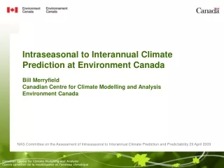
Intraseasonal to Interannual Climate Prediction at Environment Canada Bill Merryfield Canadian Centre for Climate Modelling and Analysis Environment Canada NAS Committee on the Assessment of Intraseasonal to Interannual Climate Prediction and Predictability 29 April 2009
* * Canadian Meteorological Centre (CMC) Recherche en Prévision Numérique du temps (RPN) Dorval Who we are Canadian Centre for Climate Modelling and Analysis (CCCma) Victoria
Dynamical Seasonal Forecasting in Canada • Current operational forecasts 2-tier: - 4 AGCMs x 10-ensemble (as of Oct 2007) - persisted SSTA - resolution T63 (2.8) - validated by 2nd Historical Forecast Project (HFP2) - 4-month retrospective forecasts initialized each month 1969-2003 • Forecast products: - 30 day temperature - seasonal (3-month) temperature and precip @ lead 0 and 1 month - longer term outlooks from statistical model (CCA)
Seasonal deterministic forecasts This example: temperature AMJ 2009 lead 0 months 3 category seasonal forecasts above normal normal below normal 100% 95% … historical % correct (33% = chance) 40%
90-100% Seasonal probabilistic forecasts 80-90% … This example: temperature AMJ 2009 lead 0 months prob above normal Historical reliability prob normal Observed frequency (%) prob below normal Forecast probability (%)
Development of a Coupled Forecast System ECMWF, NCEP… CCCma
Development of a Coupled Forecast System • Research network “Global Ocean Atmosphere Prediction & Predictability” (GOAPP) supported by Canadian Foundation for Climate and Atmospheric Sciences (CFCAS) • Funding to CCCma & partners Oct 2006 – Oct 2010 • CCCmapersonnel: Research Scientists • George Boer • Greg Flato • Slava Kharin (Statistics/Analysis) • Bill Merryfield (OGCM) • John Scinocca (AGCM) Research Associate • Woo-Sung Lee
Retrospective Forecasts • Pilot projectCHFP1 - initialization by simple SST nudging after Keenlyside et al., Tellus 2005 simplest procedure likely to have much skill - IPCC AR4 model CGCM3.1 - 10 member ensemble, 12 mon forecasts initialized 1 Mar, 1 Jun, 1Sep & 1Dec 1972-2001 - Skills modest as expected though competitive with 4x10 ensemble HFP2 (Merryfield et al. 2009 Atmos-Ocean, subm) • 2nd generation CHFP2 - incorporate model & initialization improvements, building on CHFP1 - Canadian contribution to WCRP/WGSIP CHFP
Coupled Forecast System Development Path CGCM development AGCM, OGCM Ocean data assimilation “Off the shelf” CGCM S assim after Troccoli et al. (MWR 2002) 2D Var after Tang et al. (JGR 2004) Improved error covariances CHFP2 CHFP1 Atmospheric initialization Simple SST nudging initialization Insertion of reanalyses Atm data assimilation Land initialization Off-line forcing by bias-corrected reanalysis + Analysis and Verification GHG forcing, trend correction, etc + Predictability
Forecast model configurations AGCM3 AGCM4 _ CHFP1 OGCM3 CHFP21 CHFP22 OGCM4 • OGCM4: higher vertical resolution (10m in upper ocean), new physics • AGCM4: many new physical parameterizations, prognostic aerosols… • Same horizontal resolution ( 2.82.8 AGCM, 1.4lon0.9lat OGCM)
Model Improvements • AGCM3 AGCM4(2.8lon x 2.8lat) - prognostic cloud scheme - improved radiation scheme - shallow convection scheme - prognostic aerosols/sulphur cycle • OGCM3 OGCM4 (1.4lon x 0.9lat) - 7 21 levels in upper 400m - KPP mixed layer - Large et al (2001) anisotropic viscosity - penetrating solar radiation (observed SeaWiFS Chl) - tidal mixing
* Monthly SSTA standard deviation Observations: HadISST 1970-99 SST Bias AGCM3+OGCM3 CHFP1 AGCM3+OGCM4 CHFP21 AGCM4+OGCM4 CHFP22
Ocean Initialization • Off-line assimilation of 3D gridded reanalyses - variational assimilation, level by level, as in Tang et al. JGR 2004* - Tang et al. used as hoc Derber & Rosati (JPO 1989) background error covariances a exp(-r2/b2)withb = 570 km - we have experimented also with covariances obtained from model variability as in Smith & Murphy JGR 2007 • S assimilation through preservation of T-S relationship - procedure of Troccoli et al. MWR 2002 - prevents spurious convection, etc. * Tang et al. obtained poor results when directly inserting T reanalyses, whereas Kirtman & Min (MWR 2009) obtained relatively good results
Salinity Correctionin Presence of T Assimilation background T-S relationship bottom Sbackground Sassim Tbackground Tassim surface
Ensemble ForecastsNino3.4 CORR from 1 Sep 1980-2001 AGCM3 + OGCM3.6
Ocean Initialization by multi-analysis assimilation • Experiment: compare NINO3.4 skill and ensemble spread for three ensemble initialization strategies: - Multi-analysis:off-lineassimilation of 6 ocean analysis products (same atm) - Exp_atmos: 6 AGCM states from consecutive days prior to forecast start (same ocn) - Exp_ocean:6OGCM states from consecutive days prior to forecast start (same ocn) • 1980-2001: 22 years of Sep 1–initialized forecasts
NINO3.4 skill and ensemble spread Ensemble Spread / RMS Error Lead month multi-reanalysis exp_atmos exp_ocean SST Forecast Skill Correlation Lines : Ensemble mean Symbols : Ensemble members Lead month Multi-analysis ocean initialization leads to • Improved skill at longer leads • Larger ensemble spread in first two months
Atmosphere Initialization • Option 1: insert NCEP reanalysis • Option 2: simple atmospheric data assimilation (IAU)
SST nudging initialzation NCEP anomalies inserted NCEP state inserted Atmosphere Initialization: NCEP Insertion 500 mb height RMS error vs time in AGCM
SST nudging initialzation NCEP anomalies inserted NCEP state inserted Atmosphere Initialization: NCEP Insertion 500 mb height RMS error vs time in AGCM AGCM assimilation?
Impact of AGCM NCEP Initialization Surface temperature correlation skill First forecast month from 1 Sep SST nudging + NCEP insertion SST nudging only
NCEP Monthly r = 0.89 NCEP Monthly r = 0.65 .95 .85 .75 .65 .55 >.5 Land surface initialization • CCCma collaboration with Aaron Berg&Gordon Drewitt (U Guelph) • Strategy: drive CLASS land surface model used in CGCM off-line with bias-corrected NCEP reanalysis after Berg et al. (Int J Clim 2005) before bias correction after bias correction correlations with gauge-based precipation
Relative soil moisture anomaly (top layer) July 2002 On-line initialization Off-line initialization
SST nudging* Forecast Combine pre-forecast AGCM, OGCM states to construct ensemble *after Keenlyside (Tellus 2005) CHFP1 initialization ensemble generation simplest procedure likely to have much skill
AGCM assim NCEP SST nudging Sea ice nudging CHFP2 initialization 3D ocean T, S assimilation or Land surface analysis Forecast ensemble generation Multiple ocean analyses and/or AGCM realizations seasonal + decadal
Ocean bias reduction through spectral nudging • Spectral nudging suppresses OGCM biases with respect to climatological mean and seasonal cycle while leaving variability on other bands unfettered • 3D Spatiotemporal filtering procedure described in Thompson et al. Ocean Modelling 2006
SST biases years 11-20 of run SSS biases conventionally nudged spectrally nudged freely running
mon SSTA standard dev years 11-20 of run mon SSTA standard dev conventionally nudged spectrally nudged freely running
Forecast Post-processing HFP2 as a laboratory for calibrating forecasts: • Kharin et al. 2009 Atmos.-Ocean in press - Skill assessment of seasonal hindcasts from the Canadian Historical Forecast Project - Probabilistic forecasts improved by fitting Gaussian vs “count” method - Examine benefits of multi-model ensembles • Boer 2009 Atmos.-Ocean in press - Climate trends in seasonal forecasts - Forecasts such as HFP2 that lack time-dependent GHG can misrepresent trends as a result - Skill can be gained by applying trend correction after the fact
N=10 4 model N=20 2 model Skill Skills of multi-model ensembles Consider all possible 1-, 2-, 3-, 4-model combinations in 4x10 HFP2 ensemble better skill for given ensemble size if multiple models Kharin et al. Atmos-Ocean 2009
Trends in seasonal forecasts Trends in SAT from NCEP and HFP2 Correlation skill score DJF NCEP Raw forecast Skill difference when trend added DJF HFP2 Boer Atmos-Ocean 2009 oC/decade
CHFP2 Seasonal forecasts Decadal forecasts 10 years 12 months WGSIP CHFP IPCC 5th Assessment (CMIP5) Conclusions • CCCma has developed coupled forecast capability from scratch over last 2-3 years CHFP2 almost ready to “fly” • Innovations include - ocean initialization with multiple reanalyses - land initialization through off-line bias-corrected forcing - spectral nudging suppresses OGCM biases without damping variability • Contribution to international CHFP • Decadal forecasts will be made for CMIP5
Conclusions • CCCma has developed coupled forecast capability from scratch over last 2-3 years CHFP2 almost ready to “fly” • Innovations include - ocean initialization with multiple reanalyses - land initialization through off-line bias-corrected forcing - spectral nudging suppresses OGCM biases without damping variability • Contribution to international CHFP • Decadal forecasts will be made for CMIP5 Intra-seasonal forecasts? CHFP2 Seasonal forecasts Decadal forecasts 10 years 12 months US Clivar Intraseasonal Prediction Experiment? WGSIP CHFP IPCC 5th Assessment (CMIP5) GLACE2?
Supplementary Slides • Model improvements • Ocean initialization • Atmosphere initialization • Land initialization • HFP2 vs CHFP1 vs CHFP2 • Forecast post-processing • Predictability
NINO3 Power Spectrum AGCM4+OGCM4 OBS 1970-99 AGCM3+OGCM3 OBS 1940-69 1 10 10-1 100 PERIOD (Y) AGCM3+OGCM3
U (lon vs depth) Temperature (lon vs depth) U at 140W (lat vs depth) Equatorial Pacific Observations: SODA AGCM3+OGCM3 CHFP1 AGCM3+OGCM4 CHFP21 AGCM4+OGCM4 CHFP22
Jan mixed layer depth Jul mixed layer depth Observations: WOA/PHC AGCM3+OGCM3 AGCM3+OGCM3 CHFP1 AGCM3+OGCM4 AGCM3+OGCM4 CHFP21 AGCM4+OGC4 CHFP22 m m
Potential for improved prediction skill with AGCM4+OGCM4 exemplified by “hit” for 11-month lead prediction of 1982/83 El Nino: Deterministic forecast SSTA Nov 1982 AGCM4 + OGCM4 Lead=11 mo Obs SSTA Nov 1982 • While such outcomes not always possible (even in theory), a strong El Nino is now within the range of possibilities admitted by the model
Error Covariance Structure Smith (colors) vs Derber-Rosati (hatched) 550m 7.5m
Correlation Lengths at Sea Surface Smith and Murphy lx (x,y) ly (x,y) CCCma Mean over Jan, Apr, Jul and Oct
Intercomparison of Ocean Reanalysis Products Time Averaged Ensemble Standard Deviation(1980-2001) 7.5m 105.5m 552.5m Depth (m) Ensemble Standard Deviation (C)
Modify Troccoli-Haines S assimilation where local preservation of T/S relation not possible
SST nudging + NCEP insertion SST nudging only Impact of AGCM NCEP Initialization Surface temperature correlation skill: Global mean 1st month improvement possible 2nd month improvement
Impact of land surface initial conditions • Land surface state (especially soil moisture) imparts predictability up to ~1 season • Land-atmosphere feedbacks concentrated in “hot spots” where soil moisture is highly variable (not too dry, not too wet) Canadian prairies Koster et al. Science 2004