Download
1 / 23
230 likes | 384 Vues
The Dynamics of Microscopic Filaments. Christopher Lowe Marco Cosentino-Lagomarsini (AMOLF). The Dynamics of Microscopic Filaments. Christopher Lowe Marco Cosentino-Lagomarsini (AMOLF). Why we’re interested: Flexible filaments are common in biology

E N D
The Dynamics of Microscopic Filaments Christopher Lowe Marco Cosentino-Lagomarsini (AMOLF)
The Dynamics of Microscopic Filaments Christopher Lowe Marco Cosentino-Lagomarsini (AMOLF) • Why we’re interested: • Flexible filaments are common in biology • New experimental techniques allow them to be • imaged and manipulated • It’s fun
are respectively the perpendicular and parallel friction coefficients of a cylinder Accounting for the fluid At its simplest, resistive force theory
Gives good predictions for the swimming speed of simple spermatozoa
F Vf Why might this not give a complete picture? A simple model, a chain of rigidly connected point particles with a friction coefficient g
F Vf Why might this not give a complete picture? A simple model, a chain of rigidly connected point particles with a friction coefficient g Ff = -g (v-vf) Vf v
The Oseen tensor gives the solution to the inertialess fluid flow equations for a point force acting on a fluid These equations are linear so solutions just add
Approximate the solution as an integral. For a uniform perpendicular force. • s = the distance along a rod of unit length • b = is the bead separation
Approximate the solution as an integral. For a uniform perpendicular force. • s = the distance along a rod of unit length • b = is the bead separation If the velocity is uniform the friction is higher at the end than in the middle
Ff Ft Fb Fx Numerical Model Fb - bending force (from the bending energy for a filament with stiffness G) Ft - Tension force (satisfies constraint of no relative displacement along the line of the links) Ff - Fluid force (from the model discussed earlier, with F the sum of all non hydrodynamic forces) Fx - External force Solve equations of motion (with m << L g / v)
Advantages • Simple (a few minues CPU per run) • Gives the correct rigid rod friction coefficient in the limit of a large number of beads if the bead separation is interpreted as the cylinder radius
Advantages • Simple (a few minues CPU per run) • Gives the correct rigid rod friction coefficient in the limit of a large number of beads if the bead separation is interpreted as the cylinder radius Disadvantages • Only approximate for a given finite aspect ratio
What happens? Sed = FL2/G = ratio of bending to hydrodynamic forces
E. Koopman presents Movie time Sed = 10
E. Koopman presents Movie time Sed = 100
E. Koopman presents Movie time Sed = 500
E. Koopman presents Movie time Sed = 1, filament aligned at 450
How many times its own length does the filament travel before re-orientating itself?
Is this experimentally relevant? • For a microtobule, Sed ~ 1 requires F~1 pN. This is • reasonable on the micrometer scale. • For sedimentation, no. Gravity is not strong enough. • You’d need a ultracentrifuge • Microtubules are barely charged, we estimate • an electric field of 0.1 V/m for Sed ~ 1
Conclusions • We have a simple method to model flexible • filaments taking into account the non-local • nature of the filament/solvent interactions
Conclusions • We have a simple method to model flexible • filaments taking into account the non-local • nature of the filament/solvent interactions • When we do so for the simplest non-trivial dynamic • problem (sedimentation) the response of the filament • is somewhat more interesting than local theories suggest
Conclusions • We have a simple method to model flexible • filaments taking into account the non-local • nature of the filament/solvent interactions • When we do so for the simplest non-trivial dynamic • problem (sedimentation) the response of the filament • is somewhat more interesting than local theories suggest • It’s just a model, so we hope it can be • tested against experiment