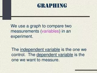
Graphing
Graphing. Required readings: graphing articles in Student Laboratory Handbook – see syllabus. Reminders and Updates. Weekly Reflection #4 due Wednesday evening. Test #1 on Thursday, February 13 th Addresses Chapters 1, 3, and 4 Faith and Knowledge Life and Times of Galileo

Graphing
E N D
Presentation Transcript
Graphing Required readings: graphing articles in Student Laboratory Handbook – see syllabus
Reminders and Updates • Weekly Reflection #4 due Wednesday evening. • Test #1 on Thursday, February 13th • Addresses Chapters 1, 3, and 4 • Faith and Knowledge • Life and Times of Galileo • Basic graphing including P-T and V-T graphs • 25 standard plus 3 extra credit M-C questions. • There is no lab this week. • There is no reading quiz for Thursday.
Review: Things you need to know… • Plotting individual points (x, y) • Regression line (best fit line) • Slope, m = Δy/Δx = (y2-y1)/(x2-x1) (include units) • y-intercept, b (include units) • Algebraic relationship: y = mx + b • Physical relationship: replace y by variable on y-axis and x by variable on x-axis • Relationships – proportional, linear, inverse, etc
Things you must be able to do… • Plot data points on a graph or read coordinates of a plotted point. • Determine and interpret the slope of a straight-line graph, including units. • Determine the y-intercept, including units. • Find a physical relationship using y=mx+b • Determine the value of a dependent variable given the value of an independent variable as well as appropriate constants.
If this is not clear… • …be certain to read “Graphing Exercises” hyperlinked to course syllabus for Tuesday, January 28th. • These “optional” readings are now required because of the loss of class time.
Test #1… General Pointers(not all inclusive) • Be sure you UNDERSTAND (not merely memorize) each of the topic areas. • Differences between ways of knowing. • Recreate solar system models and distinguish. • Know how Galileo destroyed the Ptolemaic system, but did NOT prove Earth’s motion. • Proofs for Earth’s rotation and revolution. • Create, analyze, and interpret graphs.
Rectilinear Motion Continued Sections 4.2 and 4.3
The Position-Time graph (P-T) • Slope is velocity (+/- speed) • y-intercept is position at time = 0 • y = mx + b (algebraic relationship) • distance = velocity*time + distanceo • x = vt + xowhere v = constant(equation 1) • Solving a practical problem… • In constant motion • Caution: in accelerated motion
The Velocity-Time Graph (V-T) • Slope = change in velocity / change in time which is acceleration • y-intercept equals velocity at time = 0 • y = mx + b • velocity = acceleration*time + velocityo • v = vo + at (equation 2) • Solving a practical problem…
The V-T graph details • Constant (non-accelerated) motion • Slope = zero • Uniformly accelerated motion • Slope constant, but does not equal zero • Non-uniformly accelerated motion • Slope of tangent line at a given point gives accel. • One cannot determine initial position based on a V-T graph. • The area under a V-T graph is displacement.
Uniform Acceleration in P-T Graphs • The relationship between variables in uniformly accelerated motion. • x = xo +vot + ½ at2 (Equation 3) • A practical example… • We will address this subject matter further in Chapter 6.
Kinematic Relationships • x = xo + vt (constant velocity) (equation 1) • v = vo + at (equation 2) • x = xo + vot + ½at2 (equation 3) • Substituting t from equation 2 into equation 3 results in v2 – vo2= 2aΔx (equation 4) • Extra credit project for one point: • Demonstrate the derivation of equation 4. • Turn in written proof on Thursday at start of class.