Line plots
Line plots. Plotting overview. Plotting procedures: Line plots: plot, oplot, plots, axis Map plots: contour 3-D plots: surface, shade_surf (Putting labels over the plot: xyouts ) When a plotting procedure is called, the default behavior is as follows:

Line plots
E N D
Presentation Transcript
Plotting overview • Plotting procedures: Line plots: plot, oplot, plots, axis Map plots: contour 3-D plots: surface, shade_surf (Putting labels over the plot: xyouts ) • When a plotting procedure is called, the default behavior is as follows: 1. Erase the contents of the current window (a new window is created if none exits) 2. Establish appropriate data coordinates for the input data 3. Draw axes (including labels and tick marks) 4. Draw the data lines
Line plots — Plot • Syntax: plot, x, y plot, y (the data points are plotted against corresponding array indices) plot, x, y, max=dmax, min=dmin (limit the maximum and minimum data values to be plotted) • Overplotting oplot, x, y • Scatter plots plot, x, y, psym=1 • Polar plots plot, r, t, /polar
Plot customization • Keywords General: title, charsize, charthick For data lines: linestyle, thick, psym, symsize, color, /nodata, /noerase, /noclip For axis: /ynozero, /xlog, /ylog, [xyz]title, range, style, thick [xyz]ticks, tickv, tickname, ticklen
Creating Axes • The axis procedure may be used to create customized axes on existing plots. Often used when one or more variables with different units are plotted with respect to the same ordinates axis, [x or y]axis=[0 or 1], [xy]range= …, [xy]title=… (where xaxis=0 bottom, xaxis=1 top, yaxis=0 left, yaxis=1 right) • Example: t=findgen(11) g=9.8 v=g*t x=0.5*g*t^2.0 plot, t, v, /nodata, ystyle=4, xtitle=“Time” axis, yaxis=0, yrange=[0,100], /save, ytitle=“Velocity” oplot, t, v axis, yaxis=1, yrange=[0, 500], /save, ytitle=“Distance” oplot, t, x, linestyle=2
Multiple panels and plot positioning • Global system variables • Multiple panels !p.multi=[0, n_columns, n_rows, 0, 0] To disable multiple panels: !p.multi=0 • Plot positioning !p.position=[x1, y1, x2, y2]
Graphic devices • Commonly used graphic devices: X, PS • Select a graphic device set_plot, device_name (‘X’ or ‘PS’) • Configure the graphic device device, filename=file_name, bits_per_pixel=8, /color, $ /portrait (or /landscape), $ /inches, xsize=xsiz, xoffset=xoff, ysize=ysiz, yoffset=yoff
Using fonts in postscript • See http://idlastro.gsfc.nasa.gov/idl_html_help/About_Device_Fonts.html • You can specify the name, style and size of the letters plot,[0,1] device, /times, /bold xyouts, 0.5, 0.5, ‘bold’
In-class assignment VII Data files are stored at: http://lightning.sbs.ohio-state.edu/geo820/data/ • Read the netCDF file sst.mnmean.nc for ERSST data. Plot the SST time series for 0N155E for for 1979-2005, with the corresponding y-axis on the left. • Read the HDF file ssmi.hdf. Overplot on the above figure the V10m time series for 0N155E with the corresponding y-axis on the right. • Plot four panels on the same page, with each panel containing both the SST and V10m time series for 0N155E, 0N170E, 0N185E, 0N200E