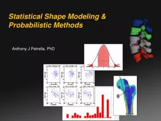
Statistical Shape Modeling & Probabilistic Methods
Statistical Shape Modeling & Probabilistic Methods. Anthony J Petrella, PhD. q. Practical Challenges in Prob Analysis. Quality deterministic model, validated How to estimate input distributions Correlated input variables

Statistical Shape Modeling & Probabilistic Methods
E N D
Presentation Transcript
Statistical Shape Modeling &Probabilistic Methods Anthony J Petrella, PhD q
Practical Challenges in Prob Analysis • Quality deterministic model, validated • How to estimate input distributions • Correlated input variables • Complex systems with long solution times require more efficient alternatives to Monte Carlo • Implementation • Matlab, Excel – simple problems • Commercial FE modules (Abaqus, ANSYS, PAM-CRASH) • NESSUS – dedicated prob code, integrates with model • Validation • Anatomical variation?
Practical Challenges • Quality deterministic model, validated • How to estimate input distributions • Correlated input variables • Complex systems with long solution times require more efficient alternatives to Monte Carlo • Implementation • Matlab, Excel – simple problems • Commercial FE modules (Abaqus, ANSYS, PAM-CRASH) • NESSUS – dedicated prob code, integrates with model • Validation • Anatomical variation? What is the best way to parameterize anatomical shape so that we can easily do Prob simulation to explore effects of anatomical variation?
Approximate with Primitives Parameterizing Anatomy • Statistical Shape Modeling (SSM) Red: m + 1*s Blue: m – 1*s (Laville et al., 2009) Lumbar (Huls et al., 2010) Hip (Barratt et al., 2008) Knee (Fitzpatrick et al., 2007)
Modeling Anatomic Variability for Application in Probabilistic Simulation of Lumbar Spine Biomechanics KS Huls, AJ Petrella, PhD Colorado School of Mines Golden, Colorado USA A Agarwala, MD Panorama Orthopaedics & Spine Center Golden, Colorado USA ICCB 2009, Bertinoro, Italy September 16-18, 2009
SSM Background 1 Training set … (N = 8) unique geometryidentical topology 2 Morph template mesh → …
SSM Background 3 remove variations intranslation & rotation retain variations insize and shape Least squares fit → (Spoor and Veldpaus, 1980) 4 Assemble data matrix →
SSM Background Principal Component Analysis = eigenanalysison covariance matrix of data, D 5 eigenvectors (cj ) = fundamental shape modes eigenvalues = variance of a each shapemode across specimens → where the bj coefficients are the “principal components”of specimen P
SSM Background 6 New virtual specimens instantiated from SSM Coefficients bj are assumed normally distributed PDF for each bj randomly sampled to instantiate any number of virtual specimens bj → …
SSM in Orthopaedics & Biomechanics • 2D kinematic measures for functional evaluation of cervical spine (McCane et al., 2006) • 3D pelvis and femur anatomy for computer-navigated total hip arthroplasty (Barratt et al., 2008) • 3D model of hemi-pelvis for use in computer-navigated THA (Meller and Kalender, 2004) • Lumbar vertebral bodies (Lorenz and Krahnstöver, 2000) • Previous work focused only on individual bones • Relative position, alignment, and conformity of articulating surfaces not considered
Objectives • Develop SSM for lumbar spine, focusing initially on the L3-L4 functional spinal unit (FSU) • Determine if virtual specimens instantiated from the SSM are biomechanically viable use finite element (FE) modeling to demonstrate normal facet articulation
Methods: Lumbar FSU • Lumbar geometry L1-L5 extracted from 8 CT data sets using Mimics software (Materialise, Inc.) • 2 Male/6 Female, 54 ± 16 yrs • Quadrilateral FE mesh created for L3 and morphed to L4 using HyperMesh software (Altair, Inc.)
Methods: Independent SSM for L3 & L4 L3 • SSM created for L3 bodies • Independent SSM created for L4 bodies • L3 and L4 bodies independently instantiated and combined to form L3-L4 functional spinal units • We refer to these models as:L3+L4 pairs L4
Methods: Unified SSM for L3-L4 • For each of the 8 specimens… • Least squares fit of L3 to L4to remove non-physiological alignment created in scanner • Unified SSM then created for L3-L4 • Virtual specimens instantiated as FSU • We refer to these models as:L3-L4 FSU
Methods: Leave-one-out Validation • Assess ability of SSM to represent the shape of an unknown specimen • Randomly selected L3 specimen removed from training data set of 8 CT scans • SSM recalculated with only seven specimens • Non-linear least squares optimization scheme was used to fit the SSM to the “left-out” specimen
Methods: FE Model • Virtual specimens created with L3+L4 SSM • Specimens also created fromSSM of the L3-L4 FSU model • ABAQUS (Simulia, Inc.) model constructed for virtual specimens • Ligaments: non-linear springs • Facet cartilage: linear elastic • Annulus: hyper-elastic matrix, linear fibers • Nucleus: incompressible fluid cavity • L4 fixed, L3 loaded with 10 N·m right axial torque
Results: Fundamental Modes of Shape • First five PC’s captured 95% of variance in data • PC1: scaling • PC2: shape and angulation of facet joints • PC3: variations in the transverse processes • Higher modes were not visually obvious Red: m + 1*s Blue: m – 1*s
Results: Leave-one-out Validation • Maximum Euclidian distance error: 5.6 mm • Mean error: 1.9 mm Red: “left out” specimen Blue: SSM fit
Results: Lumbar Model Instantiation • Appearance of virtual L3+L4 pairs • Appearance of virtual FSU specimens L3+L4-1 L3+L4-2 L3+L4-3 L3+L4-4 FSU-1 FSU-2 FSU-3 FSU-4
Results: FE Model • Facet contact area (p = 0.33)Natural: 158 ± 43 mm2FSU specimens: 120 ± 59 mm2 • Average contact pressure (p = 0.55)Natural: 0.79 ± 0.16 MPaFSU specimens: 0.88 ± 0.22 Mpa • No FE for L3+L4 specimens dueto facet interaction Natural L3+L4 FSU
Conclusions • SSM reasonable for spine, 95% of variance captured by just 5 variables • Leave-one-out validation • Errors similar to pelvis (Meller and Kalender, 2004) • Maybe acceptable for CAOS, but not for biomechanics • More specimens needed in training set • SSM instantiation • L3+L4 facet articulation not viable • FSU similar to natural facet interaction • Lumbar SSM must include all bodies to ensure reasonable inter-body articulation
SSM Summary • Why? Continuous parameterization of anatomical shape • The basic steps… • Collect data for training set • Morph to each specimen → identical topology, inter-specimen correspondence • Register specimens to common reference • Assemble data matrix • Eigenanalysis on COV matrix • Instantiate new specimens
1. Collect data for training set • Usually done with medical images • CT common for bone geometry • MR common for soft tissue, but bone extraction protocols do exist • Commercial software typically used • Mimics (Materialise) • Simpleware • Result is usually STLgeometry
2. Morph template mesh to each specimen • Essential for statistical analysis because morph creates • Identical topology • Inter-specimen correspondence – every vertex / landmark is at the same anatomical location for every specimen • Beyond the scope of our discussion, but… • Coherent Point Drift: may be used for rigid or non-rigid reg. https://sites.google.com/site/myronenko/research/cpd • Non-rigid surface registration: see class website for PDF • Other morphing studies: Grassi et al., 2011; Sigal et al., 2008; Viceconti et al., 1998
3. Register specimens to common reference • SSM quantifies variation in vertex coordinates across all specimens • Must remove variation that does not pertain to shape • Rigid registration of point sets with different topology • Coherent Point Drift – stated previously • Iterative Closest Point (ICP) – well known • From step 2: we have identical topology • Analytical registration method: Spoor & Veldpaus, 1980 based on calculus of variations, see class website for PDF
4. Assemble data matrix • Arrange each specimen in a column vector with x, y, z coordinates “stacked” as shown • Normalize to the mean specimen shape
5. Eigenanalysis on COV (C) matrix of D • Eigenanalysis equivalent to Principal Component Analysis (PCA) • Eigenanalysis of original system is tedious… • Rank = max # linearly independent col vectors • Rank of C is driven by n(specimens), not by m (data points) • Solving the alternate problem is much faster… e.g., 104 × 104 e.g., 10 × 10
6. Instantiate new specimens • Assume bi normally distributed • New specimens may be created simply with
Femur SSM Exercise • Exercise is based on a 2D femur meshed with triangular elements • See if you can build SSM and instantiate it