Download
1 / 24
240 likes | 261 Vues
A simulation study using a two-dimensional energy balance model to understand past climate changes, focusing on the Last Glacial Maximum. Explore experiments and data analysis to uncover climate mechanisms.

E N D
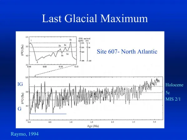
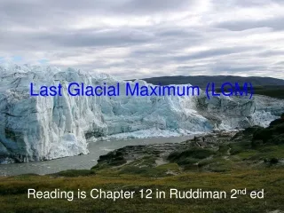
Simulation of the Last Glacial Maximum using a two-dimensional energy balance model Modeling Past and Future Climate Changes A. Paul and M. Schulz
Reading • Hartmann, D. L., 1994: Global physical climatology, Academic Press. • Section 11.6: Modeling of Ice Age Climates • Section 9.4: Ice-albedo feedback • North, G. R., Mengel, J. G. and Short, D. A.: Simple energy balance model resolving the seasons and the continents: Application to the astronomical theory of the ice ages. Journal of Geophysical Research 88, 6576-6586, 1983.
Fundamental equation • Basic assumption: everything about climate can be characterized by surface temperature • Conservation of energy in terms of • Absorbed solar energy • Emitted terrestrial energy • Energy removed by horizontal energy transport
time rate of change of the energy content of an atmosphere-ocean column of unit horizontal area = incoming solar radiation - outgoing longwave radiation - removal of energy by horizontal transport in the atmosphere and ocean
Parameterizations • Horizontal energy transport is assumed to be diffusive • Outgoing longwave radiation is assumed to be a linear function of surface temperature and a logarithmic function of the atmospheric CO2 concentration.
Discretization • The horizontal resolutionDxDy is 10°10° • 3618 grid cells • The time stepDtis about one day.
Numerical experiments • Experiment E1: control experiment, present-day land fraction, land-ice cover and CO2 • Experiment E2: glacial land-ice distribution (but still present-day land fraction) • co2ccn=280, ice_yr=-21000.0 • Experiment E3: glacial CO2 concentration • co2ccn=180, ice_yr=0.0 • Experiment E4: glacial land-ice distribution and CO2 concentration • co2ccn=180, ice_yr=-21000.0
Go to the website: http://www.palmod.uni-bremen.de/~apau/models/ebm_2d/ • Downlowd the zip-file ebm_2d_1.1.zip (1.8 MB) to your “My Documents” directory • Click on right-hand mouse button to „Extract All…“ files to a directory called: ebm_2d_1.1
Directory structure: • doc: contains the ppt file of the exercise • output: contains example MATLAB M-files (adapt to your needs) • import_data: to import model output in netCDF format • plot_data: to plot a specific variable from the model output • plot_diff: to import the model output of two experiments to plot the difference in one specific variable • global_mean: to compute the area-weighted global mean of a latitude-longitude field
work: • contains the executable program ebm_2d.exe for Windows, as well as compile scripts and a makefile if you want to build the model from the sources. • contains the parameter input file ebm.in
For all experiments, the run length runlenis taken to be 50 years (which is roughly the equilibrium timescale of the ocean mixed layer), and the time step dt is set to 1 day. • The total CPU time required for one experiment : about 13 s (for Intel Pentium 4 1.7 GHz)
Boundary conditions • Land fraction and land-ice fraction are read from file. • Surface albedo is read from file (data from McGuffie and Henderson-Sellers, zonally averaged). • Atmospheric CO2 concentration can be changed through namelist.
Land fraction - fraction of 10°10° grid cell covered by land: • 1.0 grid cell is completely land-covered, • 0.0 grid cell is completely ocean-covered.
E1/E3 • Present-day land-ice fraction - fraction of 10°10° grid cell covered by land ice: • 1.0 grid cell is completely land ice-covered, • 0.0 grid cell is completely land ice-free.
E2/E4 • LGM land-ice fraction - fraction of 10°10° grid cell covered by land ice: • 1.0 grid cell is completely land ice-covered, • 0.0 grid cell is completely land ice-free.
Exercise • Carry out experiments E1 to E4, one after the other. • Prepare a table that lists the global-mean temperature for each experiment. • Plot the time-averaged sea-level air temperature for each experiment, as well as the change from one experiment to the next. • Describe characteristic features (maximum changes, patterns) of the temperature anomalies. • Key question: From your series of experiments, which mechanism makes ice ages simultaneous in both hemispheres?
Experimental procedure • To run the model, first double-click on start_cygwin • To check and change the model parameters, type notepad ebm.in & on the cygwin commandline and press <enter>. • For your first experiment “E1”, set ice_yr to 0.0 and co2ccn to 280.0. • To start the model, type ebm_2d on the cygwin command line and press <enter>. • Upon completion of the run, the model outputs the total number of time steps performed ittmax, the number of time steps per year ntyear and the area-weighted global mean temperature at the end of the experiment in °C tgmean.
After running the model, rename the output file. • For example, from snapshot_ebm.nc to snapshot_ebm_E1.nc • Visualize the output using MATLAB. • Alternatively, you could use ferret or Panoply. • To prepare the next experiment, change the input parameter(s) in the file ebm.in accordingly • For example, change ice_yr from 0.0 to -21000.0
Sample MATLAB session • Start MATLAB. • Point “Current Directory” to output (the full path name is probably: C:\Documents and Settings\geo\My Documents\ebm_2d_1.1\output) • Take the time to inspect the M-files provided in the MATLAB editor (you can open them using File > Open). • Initialize all MATLAB paths by typing start in the “Command Window”. • Import the model output using: import_data • This M-file script lists the variables contained in the model output file (see table). • To plot, e.g. the time-averaged sea-level air temperature ta_at, try: plot_data. • If you want to plot a different variable, edit the M-file script plot_data.m accordingly, or use the MATALAB Command Window.
To plot the temperature difference between two experiments, inspect the M-file script: plot_diff.m • To compute the area-weighted global mean of a latitude-longitude field like ta_at, use global_mean(xt,yt,ta_at)
Sample ferret session • Double_click start_ferret in output folder • Type ferret and press <enter> • Type use snapshot_ebm (and press <enter>) • To shade sea-level air temperature: type shade ta_at • To compute global-mean temperature: type list ta_at[x=@ave,y=@ave]
Differences to text book example • Experiment missing with respect to Section 11.6 by Hartmann (1994): Change in snow-free surface albedo that would correspond to the land conditions for the last glacial age • associated with changes in the vegetation and soil • Furthemore, 2D EBM does not contain explicit „50-m-deep mixed-layer ocean“, which would allow the prediction of SST.