Download
1 / 19
190 likes | 341 Vues
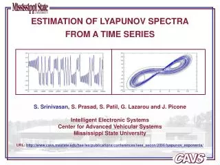
Estimation of Lyapunov Spectra from a Time Series. S. Srinivasan, S. Prasad, S. Patil, G. Lazarou and J. Picone Intelligent Electronic Systems Human and Systems Engineering Department of Electrical and Computer Engineering. Overview. What is Chaos?

E N D
Estimation of Lyapunov Spectra from a Time Series S. Srinivasan, S. Prasad, S. Patil, G. Lazarou and J. Picone Intelligent Electronic Systems Human and Systems Engineering Department of Electrical and Computer Engineering
Overview • What is Chaos? • Deterministic chaos or stochastic noise: Similarity and distinction between chaos and noise • Characterization of chaotic signals: Lyapunov exponents, entropy, dimension • Reconstructed Phase Space (RPS) • Embedding: usingderivatives, integrals, time-delay, Singular Value Decomposition (SVD) • Time delay and SVD embedding • Lyapunov Exponents (LE’s) and their Computation • What LE’s mean? • Computation of Lyapunov exponents • Experiments and results: Lorentz, Rossler, Sine
What is Chaos? • What is Deterministic Chaos? • Chaos: Sensitivity to initial conditions • Deterministic Systems: Every event is the result of preceding events and actions; events completely predictable, at least, in principle • Chaos says: ONLY in principle • Deterministic Chaos or Stochastic Noise? • Both have continuous power spectrum: not easily distinguishable • Noise is infinite-dimensional: infinite number of modes • Chaos (or deterministic noise) is finite dimensional: Dimension no longer associated with number of independent frequencies, but a statistical feature related to both temporal and geometric aspect
What is Chaos? • Characterization of Chaotic Systems • Invariants of the system • System Attractor: Trajectories approach a limit – point, limit cycle, torus, and strange. • Geometry of Strange Attractor: Scale laws characterizing self similarity (fractal dimension), correlation dimension • Temporal Aspect of Chaos: Characteristic exponents or Lyapunov Exponents (LE’s) - captures rate of divergence (or convergence) of nearby trajectories; Entropy • Any characterization presupposes that phase-space is available. What if only one scalar time series measurement of the system is available?
Reconstructed Phase Space (RPS) • Embedding • Map one-dimensional time series to a m-dimensional series • Taken’s theorem: (under some conditions) Can construct an RPS “equivalent” to the original phase space by embedding with m ≥ 2d+1 (d is the system (Hausdorff) dimension) • Dimension from Taken’s theorem: only a theoretically sufficient (but not necessary) bound. Embedding with lesser dimensions suffice in practice • Equivalent: means the system invariants characterizing the attractor is the same • Equivalent: does not mean RPS is original phase space • How to build RPS: differential embedding, integral embedding, time delay embedding, SVD embedding
Reconstructed Phase Space (RPS) • Time Delay Embedding • Uses delayed copies of the original time series as components of RPS to form a matrix • m: embedding dimension, : delay parameter • Each row of the matrix is a point in the RPS
Reconstructed Phase Space (RPS) • Time Delay Embedding • Too small value for delay parameter: leads to highly correlated vector elements, concentrated around the diagonal in embedding space. Structure perpendicular to the diagonal not captured adequately • Too large value for delay parameter: leads elements of the vector to behave as if they are independent. Evolutionary information in the system is lost • Quantitative tools for fixing delay: Plots of autocorrelation and auto-mutual information are useful guides • Advantages: Easy to compute; the attractor structure is not distorted since no extra processing is done on it • Disadvantages: Choice of delay parameter value is not obvious; leads to poor RPS in presence of noise
Reconstructed Phase Space (RPS) • Singular Value Decomposition (SVD) based Embedding • Works in two stages: • Delay embed, with one sample delay, to a dimension larger than twice the actual embedding dimension • Reduce this matrix using SVD to finally have number of columns equal to embedding dimension • SVD window size: dimension of time delayed embedded matrix over which SVD operates • Advantages: No delay parameter value to be set; more robust to noise due to SVD stage • Disadvantages: Noise reducing property of SVD may also distort the attractor properties
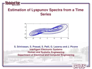
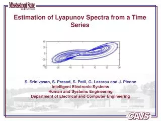
Reconstructed Phase Space (RPS) Attractor reconstruction using SVD embedding (for a Lorentz sysem)
Lyapunov Exponents and their Computation • Lyapunov Exponents • Analyzes separation in time of two trajectories with close initial points • Quantifies this separation, assuming rate of growth (or decay) is exponential in time, as: • where J is the Jacobian matrix at point p.
Lyapunov Exponents and their Computation • Properties of Lyapunov exponents • m-dimensional system has m LE’s • LE is a measure averaged over the whole attractor • Sum of first k LE’s: rate of growth of k-dimensional Euclidean volume element • Bounded attractor: Sum of all LE’s exponents equal zero or negative • Zero exponents indicate periodic (limit cycle) attractor or a flow • Negative exponents pull points in the basin of attraction to the attractor • Positive exponents indicate divergence: signature for existence of chaos
Lyapunov Exponents and their Computation • Algorithm for Computation of LEs • Embed time series to form RPS matrix. Rows represent points in phase space • Take first point as center • Form neighborhood matrix, each row obtained by subtracting a neighbor from the center • Find evolution of each neighbor and form the evolved neighborhood matrix by subtracting each evolved neighbor from the evolved center • Compute trajectory matrix at the center by multiplying pseudo-inverse of neighborhood matrix with evolved neighborhood matrix • Advance center to a new point and go to step 3, averaging the trajectory matrix in each iteration • The LEs are given by the average of the eigenvalues from each R matrix. Direct averaging has numerical issues, hence an iterative QR decomposition method (treppen-iteration) is used.
Experimental Setup and Results • Experimental Setup • Three systems tested : two chaotic (Lorentz and Rossler) and one deterministic (sine signal) • Two test conditions: clean and noisy (10 dB white noise) • Lorentz system: • Parameters: • Expected LEs: (+1.37, 0, -22.37) • Rossler system: • Parameters: a = 0.15, b = 0.2, c = 10 • Expected LEs: (0.090, 0.00, -9.8) • Sine Signal: • Parameters: Freq=1Hz, Samp freq=16Hz, Amp=1 • Expected LEs: (0.00, 0.00, -1.85)
Experimental Setup and Results • Experimental Setup • 30000 points were generated for each series in both the conditions • 5000 iterations (or the number of evolution steps) were used for averaging using QR treppen-iteration • Variation of LEs with SVD window size and number of nearest neighbors • Varied number of neighbors with SVD window size as 15 in clean and 50 in noisy condition • Varied SVD window size with number of neighbors as 15 in clean and 50 in noisy condition
Experimental Setup and Results LEs from Lorentz System
Experimental Setup and Results LEs from Rossler System
Experimental Setup and Results LEs for Sine Signal
Experimental Setup and Results • Results • In clean condition: Positive and zero exponents are almost constant at the expected values for all three test signals • In noisy condition: Positive and zero exponents converge to the expected value for SVD window size about 50 and number of neighbors also about 50 • Negative exponent: In all cases it is unreliable, but it is least useful of the exponents in chaos
References • References • [1]J. P. Eckmann and D. Ruelle, “Ergodic Theory of Chaos and Strange Attractors,” Reviews of Modern Physics, vol. 57, pp. 617‑656, July 1985. • [2] M. Banbrook, “Nonlinear analysis of speech from a synthesis perspective,” PhD Thesis, The University of Edinburgh, Edinburgh, UK, 1996. • [3] E. Ott, T. Sauer, J. A. Yorke, Coping with chaos, Wiley Interscience, New York, New York, USA, 1994