Introduction to Medical Imaging Techniques: From X-Rays to Dual-Energy X-Ray Absorptiometry (DXA)
520 likes | 784 Vues
Explore the principles and applications of various medical imaging techniques, from conventional radiography to advanced CT and DXA methods. Learn about detectors, acquisition processes, and quantification methods in the field of medical imaging.

Introduction to Medical Imaging Techniques: From X-Rays to Dual-Energy X-Ray Absorptiometry (DXA)
E N D
Presentation Transcript
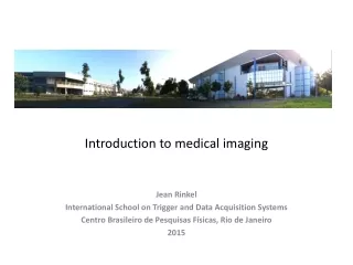
Introduction to medical imaging Jean Rinkel International School on Trigger and Data Acquisition Systems Centro Brasileiro de PesquisasFísicas, Rio de Janeiro 2015
Outline X-rays Radiography Computed Tomography (CT) Single Photon Emission Tomography (SPECT) Positron Emission Tomography (PET) Non-ionizing radiation techniques Magnetic Resonance Imaging (RMI) Echography Medipix detectors
Medical imaging modalities Source: Winnie Wong International School on Trigger and Data Acquisition Systems Wigner Datacenter Budapest, 2014
Principle of Radiography X-ray production Image source: The Essential Physics of Medical Imaging (textbook) Image source: http://www.arpansa.gov.au/radiationprotection/basics/xrays.cfm Interactions of X-rays with Matter Beer-Lambert attenuationlaw: Measured spectrum N(E) Incident spectrum N0(E) T L mat • Trade-off to set the energy: • High variability of τmatto separate soft issues at low energies • High dose to patient at low energies
Detectors in Radiography Conventional radiography (Films) • Based on a layer of light-sensitive emulsion consisting of silver halide (about 95% AgBr and 15% AgI) • When interacting with x-rays, Br- ions are liberated and captured by the Ag+ ions. • Process of developing with a chemical to form metallic silver (black) http://medinfo.ufl.edu/other /histmed/klioze/index.html Analysis limited to qualitative visual interpretation • Computed radiography • Absorbed x-ray energy is trapped in a photostimulable phosphor (PSP) screen(usually BaFBr) • The imaging plate is run through a special laser scanner, or CR reader, that reads and digitizes the image • Can be reused Main drawback: slow readout process Image source: The Essential Physics of Medical Imaging (textbook)
Detectors in Radiography Digital radiography: flat panel detectors with real time display Direct conversion - Photoelectric absorption of the X-ray photons within the sensor (semi conductor, usually Amorphous selenium, a-Se – other materials tested: Si, CdTe, Ge) - Ion pairs are collected under applied voltage across the solid state converter Indirect conversion Flat panel detectors based on scintillators layer (usually caesium iodide (CsI) or gadolinium oxysulfide (Gd2O2S)) combined with a-Si photodiodes Trixell flat panel detector 3200×2304 pixels - Numerical detectors furnish an information which can be directly post processed - Enables quantification
Detector T Scatter Incident beam Direct beam Compression paddle Quantification in mammography Objective Estimate an image of the mass composition of the two main components of breast soft tissues (fat and glandular tissues) to optimize breast cancer detection Acquisition Breast compression to ensure a constant thickness T Breast Data processing 1) Direct problem Thickness equation: X-ray measurement: 2) Per pixel inversion With the monochromatic approximation:
Rough mammogram Thickness of glandular tissue Quantification in mammography
Dual-energy X-ray absorptiometry (DXA) Principal application: measurement of bone mineral density (BMD), reflecting the strength of bones as represented by calcium content Incident Flux (energy E) Projected mass (g/cm2) Mass attenuation coefficient Bone(b) / Soft tissue (st) Transmitted flux Attenuation Measurements at 2 energies (L, H) Reconstruction
1mm Al 2mm Al 3mm Al 4mm Al Dual-energy X-ray absorptiometry (DXA) Two approaches to generate the two energies: kVp and filter switch or only filter switch Polychromatic spectra: Example of Low Energy spectra
Dual-energy X-ray absorptiometry (DXA) Polychromaticity Non linear direct problem Inversion by deformation of the linear approach: Calibration to estimate the coefficients of the polynomial
Dual-energy X-ray absorptiometry (DXA) Low energy acquisition High energy acquisition Combination Bone mineral density Soft tissues
Dual-energy X-ray absorptiometry (DXA) Low energy acquisition BMD image Soft tissues image Arm Hip Backbone
Lowenergyacquisition High energyacquisition Dual-energy X-ray absorptiometry (DXA) Thoracic radiography BMD Soft tissues
Dual-energy X-ray absorptiometry (DXA) Encephalometry BMD zoom Low energy acquisition Soft tissues
Introductiontocomputedtomography(CT) Outline Introduction Radiography CT SPECT PET Medipix • History • First CT scanner in 1972 (EMI) • Hounsfield awarded by the Nobel prize in Physiology or Medicine 1979 • 4 minutes /scan Principle “Tomography” refers to a picture (graph) of a slice (tomo). Radiography : projection on a plane of superposition of anatomical structures CT: combination of various radiography at different angles to eliminate this superposition and display three-dimensional (3D) slices Units Radiography: attenuation Tomography: linear attenuation coefficient μ (3D map) Image source: The Essential Physics of Medical Imaging (textbook) Hounsfield units:
Dose in CT http://www.radiologyinfo.org/en/safety/?pg=sfty_xray
Detectors in CT Indirect conversion: Image source: The Essential Physics of Medical Imaging (textbook)
Generations of CT Second generation: - Narrow beam irradiating a few detectors (up to 30) - For each slice: translation + rotation of the system « source + detectors » - Duration of scan (average): less than 90 s First generation: - One source and one detector - Pencil-like X-ray beam - For each slice: translation + rotation of the system « source + detector » - Duration of scan (average): 25-30 mins Fourth gneration: - Detectors: multiple (more than 2000) arranged in an outer ring which is fixed - The source only is rotating - Duration of scan (average): few seconds Third generation: - Suppresion of the translation - Broad beam covers the whole volume of the patient - Until 700 detectors - For each slice: rotation of the system « source + detector » - Duration of scan (average): approximately 5s http://perso.telecom-paristech.fr/~bloch/ATIM/tomo.pdf Evolution of acquisition time: 5 minutes / slice in 1972 vs 0.35 s / rotation today
Multislice CT – dose andacquisition time Number of pixel rows tend to increase (in the z-axis) -> Reduced acquisition time Image source: The Essential Physics of Medical Imaging (textbook) -> Reduced dose due to the z-axis geometric efficiency http://www.impactscan.org/download/msctdose.pdf Today: most fabricants propose 64 slices scanners
1 strip- 1972 (EMI) Multislice CT andscatter Effect of detector size Evolution of detector size X-ray source Volume of the patient producing scatter X-ray source Volume of the patient producing scatter 64 strips- 2004 (Toshiba)
4.5 4 3.5 3 2.5 2 1.5 1 0.5 0 Scatter image Transmitted image Multi slice CT and scatter Incident X-rays flux = + Image of transmitted beam Image of scatter Acquired image Patient
Multi slice CT and scatter correction Source: Phys. Med. Biol. 52 (2007) 4633–4652
Classical reconstruction in CT Radon transform and sinogram t pq(t) y t u q x f Reconstruction: inversion of the Radon transform - finding f(x,y) fromPq(t) Filter back projection algorithm (FBP): Ramp Filter • Exact • Fast • Not well adapted for noisy data 24 0
Iterative reconstruction in CT Standard FBP vs iterative reconstruction Example of the MLEM (Maximum Likelihood Expectation Maximization) algorithm The image at the iteration k+1, fik+1, is estimated by multiplying the previous image, fik, by a correction factor: • pj: measured projection • Rji radon transform operator • The correction factor is the normalized retroprojection of the measured projection divided by the calculated projection Bayesian algorithm: optimizes the likelihood of the estimated image knowing the measurement under the hypothesis of a Poisson noise. Dushyant Sahani, Iterative Reconstruction Techniques (ASIR, MBIR, IRIS): New Opportunities to Lower Dose and Improve Image Quality SCBT-MR 2015
Multislice CT – iterativereconstruction Recent Integration of iterative reconstruction methods: GE: ASIR (Adaptive Statistical iterative Reconstruction) - 2009 Siemens: IRIS (Iterative Reconstruction in Image Space) - 2010 Philips: iDose - 2011 Toshiba: AIDR (Adaptive Iterative Dose Reduction) - 2011 Dushyant Sahani, Iterative Reconstruction Techniques (ASIR, MBIR, IRIS): New Opportunities to Lower Dose and Improve Image Quality SCBT-MR 2015 American Journal of Roentgenology. 2010;195: 713-719
Dual energy CT • Quick kV switch to achieve dual energy acquisition in a single acquisition • Dual source CT Dual-energy tomography vs Subtraction angiography (invasive technique) Source: Acad Radiol 2012; 19:1149–1157
Single photon emission computed tomography (SPECT) Outline Introduction Radiography CT SPECT PET Medipix • Injection of gamma emitting radionuclide into the patient with specific binding to certain types of tissues • Gamma-ray detection by a nuclear camera of emissions from the patient from a series of different angles around the patient (Typically: 1282 pixels with120 or 128 projection images) • Tomographic reconstruction of emission images • Functional information: distribution of the radioactive agent Typical 180-degree cardiacorbit RAO (right anterior oblique) to LPO (left posterior oblique) Parallel collimation Trade-off between spatial resolution and the detection efficiency Spatial resolution depends strongly on the collimator and the source position. Typical values for low-energy high-resolution parallel hole collimators : - Tangential resolution for the peripheral sources :7 to 8 mm FWHM - Central resolution: 9.5 to 12 mm - Radial resolution for the peripheral sources: 9.4 to 12 mm
Positron Emission Tomography (PET) • Principle: detection of pairs of gamma rays emitted indirectly by a positron-emitting radionuclide. • - The emitted Positron scatter through matter • It annihilates with an electron resulting in two 511-keV photons emitted in opposite directions • Simultaneous detection means that an annihilation occurred on the line connecting the two detectors Radionuclide: Example of active molecule: fluorodeoxyglucose (FDG): analog to glucose indicate the tissue metabolic activity explore the possibility of cancer metastasis Detectors • Comparison to SPECT: • Better spatial resolution: typically 5-mm FWHM in the center of the detector ring • PET usually more expensive than SPECT scans: able to use longer-lived more easily obtained radioisotopes than PET. Typical time windows - BGO detectors: 12 ns - LSO detectors: 4.5 ns
Dual modality (SPECT / CT and PET CT) Simultaneous acquisition of PET or SPECT and low dose CT: - CT provides - good depiction of anatomy - attenuation correction - help for patient alignement - SPECT or PET provides functional information Example of PET CT images: PET information superimposed in color on grayscale CT images Source: http://www.chups.jussieu.fr/ext/OLDceb/protected/protectedCNEBMN/atelierDreuilleTEP/ArticleEMC_PET.pdf
Time Counting 30 keV 1 - 1 s(t) - 1 1 Spectroscopy 1 1 1 1 1 1 1 1 1 1 1 1 ΔT Charge time threshold 90keV 80keV s(t) 70keV Counting 60keV 60keV 60keV 50keV 50keV 30keV 40keV 30keV 40keV 20keV 30keV 20keV 10keV ΔT time Spectroscopy Direct conversion detectors Outline Introduction Radiography CT SPECT PET Medipix Pitch Anodes Semi condutor Cathode Photon
Medipix overview Outline Introduction Radiography CT SPECT PET Medipix • Medipix3 Timepix3 • Pixel size: 55x55um • Format 256x256= 65536px • Framing rate: 1000Hz http://medipix.web.cern.ch/medipix/pages/medipix3.php • Medipix3 (Frame based) • Single pixel mode: High dynamic range (24 bits) • Charge summingmode (12 bits) • Spectrometricmode: 110 μm pixels / 8 energythresholds (12 bits) • Timepix3 (Data-driven) • Counting • Time over Threshold (ToT) • Time of Arrival (ToA) Source: T. Poikela et al, 15th INTERNATIONAL WORKSHOP ON RADIATION IMAGING DETECTORS, 2013
Tomography at the brazilian synchrotron Micro tomography based on indirect conversion (scintillator + CCD) Direct conversion (Medipix) • Best signal to noise ratio compared to classical systems • Counting • Higher efficiency • Lower spatial resolution • Pixel size limited by the CMOS technology 130 nm • Charge sharing effect Counting rate • Cellular structure and features • Cell types and orientation • Biology 1mm 1mm
Toward spectral tomography Timepix used at 3 different threshold positions: between and after K edges of Cd and Cu Source: Enrico Jr Schioppa et al 2012 JINST7 C10007
Conclusion Through examples of medical applications using ionizing radiation: • Quantification approaches enabled by emergence of numerical detectors (combined with applied mathematics and calibration procedures) • Recent innovations to optimize acquisition time and dose for a given image quality and associated problems and limitations: • Multi slice CT • Direct conversion (example of Medipix and Timepix) • Suggested reading • Books: • J.Bushberg et al., The EssentialPhysicsof Medical Imaging, 3rd Ed., 2012 • J. Jan, Medical ImageProcessing, ReconstructionandRestoration, ConceptsandMethods, 2006 • Medipix: • - http://medipix.web.cern.ch/medipix/
Project of module based on 12 Medipix3RX Pilatus 100k Dectris detector Pixel 172 x 172 μm2 Area 28cm2 Number of Pixels 95K pixels Pixel 55 x 55 μm2 Area 24cm2 Number of Pixels 786K pixels Possibility to add various modules (3 modules equivalent in size to Pilatus 300k) http://photon-science.desy.de/research/technical_groups/detectors/projects/lambda/index_eng.html
Project of module based on 12 Medipix3RX Single chip inputs / outputs 8 LVDS pairs receivers 10 LVDS drivers (8 for data) 2 analog inputs (generated from DACs) 1 analog output (to be connected to an ADC) Full parallel readout of 12 chips: 161 LVDS pairs (using 8 lines in parallel /chip for data) 24 analog inputs 12 analog outputs • Main numbers: • - Total Readout time (12 chips Medipix3RX / 24bits counters and 350MHz) = 562 us • Frame rate (for acquisition time = 10% of readout time) = 1615 f/s • Required Bandwidth: 7.6 Gbytes/s • 2.4 Mbytes images
Project with NI PXI-7952R 1 main board + 9 adapters Communication and powering of 9 Timepix chips + synchronization with external equipments Detector 1 . . . Detector 9 Adaptor 1 . . . Adaptor 9 MainBoard
Project with NI PXI-7952R Objective: full parallel readoutof 9 chips Medipix3RX / TIMEPIX connected to one NI PXI-7952R Limitation =>Maximum number of LVDS pairs data outputs : 1 (instead of 8 in an optimized configuration) with 66 LVDS pairs Main numbers: - Total Readout time (9 chips Medipix3RX / 24bits counters and 350MHz) = 4.5 ms - Frame rate (for acquisition time = 10% of readout time) = 202 f/s - Required bandwidth: 715 Mbytes/s - 1.8 Mbytes images
Comparison and conclusion PROJECT WITH 12 CHIPS 12 786.432 24,0 cm² Parallel 8 lines / 24bits 563 us 1615 f/s 2,4 MB 161 24 12 7.6 GB/s DETECTOR OF SAME AREA THAN PILATUS 6M 840 55.050.240 1.680,0 cm² Parallel 8 lines / 24bits 563 us 1615 f/s 165,1 MB 11.270 1680 840 532 GB/s PROJECT WITH NI 7952R 09 589.824 18,0 cm² Parallel 1 line / 24bits 4,5 ms 202 f/s 1,8MB 59 0 1 715 MB/s Number of chips Number of pixels Total area Operation mode Readout time Frame rate Image size LVDS pairs Analog inputs Analog output Transfer rate • For National Instrument solution being competitive with 12 chips project: • Need for a Board with 161 LVDS pairs • Data have to be transmitted without lost through long flat cables (a few meters) at 350 MHz • On-board memory: 2,4 MB - 7.6 GB/s