Download
1 / 20
200 likes | 255 Vues
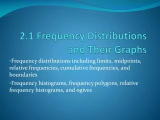
Learn how to create grouped and ungrouped frequency distributions for quantitative variables, and explore various graphs for visualizing data effectively. The course covers constructing histograms, frequency polygons, cumulative distributions, and stem-and-leaf displays. Understand the conventions, benefits, and drawbacks of grouping data, along with interpreting relative and cumulative frequency distributions. Gain insights into constructing frequency distributions for qualitative variables and graphs such as bar graphs and pie charts. Avoid common pitfalls like misleading graphs and learn how to present data accurately. Enhance your statistical analysis skills with practical examples and techniques in this comprehensive guide.

E N D
Chapter 2 • Frequency Distributions and Graphs • I Frequency Distributions for Quantitative Variables • A. Ungrouped Frequency Distribution • 1. Each class interval contains a single score value
Table 1. Taylor Manifest Anxiety Scores • (1) (2) 74 1 73 1 72 0 71 2 70 7 69 8 68 5 67 2 66 1 65 1 n = 28
2. Class interval size, i i = score real upper limit – score real lower limit B. Grouped Frequency Distribution 1. Each class interval spans two or more score values
Table 2. IQ Data (1) (2) Xjf 160–169 1 150–159 1 140–149 0 130–139 2 120–129 3 110–119 6 100–109 8 90–99 3 80–89 1 70–79 1 n = 26
C. Conventions Used in Constructing Frequency Distributions D. Determining the Number and Size of Class Intervals By Trial and Error E. Pros and Cons of Grouping Data
F. Relative Frequency Distributions Table 3. IQ Data (1) (2) (3) (4) Xj f Prop f % f 160–169 1 .04 4 150–159 1 .04 4 140–149 0 .00 0 130–139 2 .08 8 120–129 3 .12 12 110–119 6 .23 23 100–109 8 .31 31 90–99 3 .12 12 80–89 1 .04 4 70–79 1 .04 4 n = 26 1.00 100
G. Cumulative Frequency Distributions Table 4. IQ Data (1) (2) (3) (4) (5) (6) Xjf Prop f % f Cum prop f Cum % 160–169 1 .04 4 1.00 100 150–159 1 .04 4 .98 98 140–149 0 .00 0 .94 94 130–139 2 .08 8 .94 94 120–129 3 .12 12 .86 86 110–119 6 .23 23 .74 74 100–109 8 .31 31 .51 51 90–99 3 .12 12 .20 20 80–89 1 .04 4 .08 8 70–79 1 .04 4 .04 4 n = 26 1.00 100
II Frequency Distribution for Qualitative Variables Table 5. Leading Cause of Death of Men in 2006 XProp f Accidents .07 Cancer .22 Heart disease .38 Stroke .08 Other .25 Total 1.00
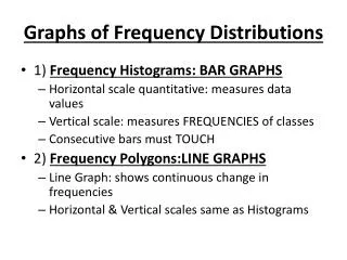
A. Conventions Used in Constructing Frequency Distributions for Qualitative Variables III Graphs for Quantitative Variables A. Histogram for IQ Data
D. Stem-and-Leaf Display for IQ Data • (1) (2) (3) • StemsLeaves f • 70–79 8 1 • 80–89 5 1 • 90–99 3 8 6 3 • 100–109 7 1 8 2 9 5 4 3 8 • 110–119 6 2 3 5 6 8 6 • 120–129 2 9 7 3 • 130–139 3 5 2 • 140–149 0 • 150–159 2 1 • 160–169 0 1
IV Graphs for Qualitative Variables A. Bar Graph for Leading Cause of Death of Men in 2006
1. Construction of pie charts Conversion of Prop f To Minutes Accidents .07 60 = 4.2 Cancer .22 60 13.2 + 4.2 =17.4 Heart disease .38 60 22.8 + 17.4 = 40.2 Stroke .08 60 4.8+ 40.2 =45.0 Other .25 60 15.0+ 45.0 =60.0
VI Misleading Graphs Figure 1. Two plots of the same data. Figure (a) is misleading.
A. Pictogram Figure 2. Figure (a) is misleading because it uses both height and area to represent computer sales