Download
1 / 37
440 likes | 789 Vues
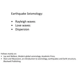
Earthquake Seismology: Rayleigh waves Love waves Dispersion. Follows mainly on: Lay and Wallace, Modern global seismology, Academic Press. Stein and Wysession , an introduction to seismology, earthquakes and Earth structure, Blackwell Publishing.

E N D
Earthquake Seismology: • Rayleigh waves • Love waves • Dispersion • Follows mainly on: • Lay and Wallace, Modern global seismology, Academic Press. • Stein and Wysession, an introduction to seismology, earthquakes and Earth structure, Blackwell Publishing
Seismologist measure the seismic waves near the free-surface, and it is thus important to understand the near surface effects: • At the surface, both incident and reflected waves coexist, and the total amplitude is the sum of the two. • SH waves do not interact with the P and SV waves at the free-surface. • The interaction between P and SV waves with the free-surface gives rise to an interference waves that travel along the surface as Rayleigh waves.
RAYLEIGH WAVES The existence of Rayleigh waves was predicted in 1885 by Lord Rayleigh, after whom they were named.
RAYLEIGH WAVES Boundary conditions: 1) For surface waves to be trapped near the surface, the energy must decay with depth. 2) Free-surface is traction free. Since the SH wave does not interact with the P and SVwaves at the surface, it is ok to disregard the former. The P and Sv potentials are: The wave numbers kxand kz are not independent, but are related through the wave speeds.
RAYLEIGH WAVES The following sketch illustrates how kx, kz and the wave speeds are related: We get that: * For P-wave: * For S-wave:
RAYLEIGH WAVES The requirement that the surface wave energy would decay with depth is satisfied if: Thus, cx, the apparent velocity along the surface, is less than the shear velocity. It is convenient to define: Substituting these into the potentials gives:
RAYLEIGH WAVES The next requirement that we seek to satisfy is that the tractions vanish at the free-surface. That is: Recall that the displacements in terms of potentials are: Replacing these into Hooke’s law gives:
RAYLEIGH WAVES The solution of which is: Replacing ra and rb with and ,respectively, and using the relation between the Lame constants and the wave speeds gives: Or alternatively, in a matrix form:
RAYLEIGH WAVES To find the non-trivial solutions, we set the determinant to be equal zero: If the medium is Poissonian, a2/b2=3, and the determinant becomes: There are 4 roots to this polynom (see p. 88 in Stein and Wysession): Only the last solution satisfies the requirement that: And we conclude that (for Poissonian solid) the Rayleigh wave speed is slightly less than the shear wave speed (~0.92b).
RAYLEIGH WAVES The result that: can now be used to find the coefficients of the potentials (A and B) and the displacements (ux,uz).
RAYLEIGH WAVES Particle motion diagrams. Plots illustrate the particle motion by plotting seismograms for two components of motion. Source: http://web.ics.purdue.edu/~braile/isw/motion_files/image002.jpg
RAYLEIGH WAVES Particle motion (velocity in radial–vertical plane) in the Rayleigh wave during 1.5 sec (starting 5.1 sec after P-wave arrival) for the mining event MN 2.1, 5 August 2008, in the 0.2–4.0 Hz frequency band at various depths. Arrows show direction of particle motion. Source: Atkinson and Kraeva, 2010.
LOVE WAVES Augustus Edward Hough Love predicted the existence of Love waves mathematically in 1911 (Chapter 11 from Love's book "Some problems of geodynamics", first published in 1911). Love waves travel with a slower velocity than P- or S- waves, but faster than Rayleigh waves.
LOVE WAVES • Result from the interaction of SH waves. • Require a velocity structure that varies with depth, i.e., cannot exist in a homogeneous half-space. • Require that b2>b1.
LOVE WAVES Boundary conditions: 1) For surface waves to be trapped near the surface, the energy must decay with depth. 2) Free-surface is traction free. 3) Displacement and stress continuity at the interface between the layer and the half-space.
LOVE WAVES The uy displacement in the layer is: and within the half-space: To obtain B1, B2 and B’, we use the boundary conditions at the free-surface and the interface of the half-space. At the free-surface: Therefore at z=0, B2=B1.
LOVE WAVES At z=h, the displacement is continuous for all x and t: and so is the stress: By writing the complex exponentials as a sum of sines and cosines, we write (1) and (2) as: 1a. and: 1b. Next, we divide (1b) by (1a). 1. 2.
LOVE WAVES Dividing (1b) by (1a) from the previous slide gives: with . The above equation may be rewritten as a function of any two of the three parameters: cx,w and kx. Writing the above in terms of cx and w yields: Because the tan function gives real values, the square roots must be real, and therefore the apparent velocity is bounded as: * See box on next page
LOVE WAVES Taken from Stein and Wysession, p. 90-91
LOVE WAVES It is useful to define a new variable: Because the apparent velocity ranges between b1 and b2, we get that: We get:
LOVE WAVES Here’s a graphical solution of this result for different frequencies: • Solutions exist where the two curves intersect. • These solutions are called modes. • For a given frequency there are several modes, each with different apparent velocity. • The leftmost solution, with the lowest cx is called the fundamental mode, and the other are the overtones.
LOVE WAVES • For sufficiently longperiods, only the fundamental mode exist. • At shorter periods, higher modes exist. • The longest period at each branch approaches the velocity of the half-space, i.e. it is unaffected by the velocity of the top layer. • For a given branch, apparent velocity increases with period.
LOVE WAVES • Variations in the apparent velocity are due to differences in displacement profiles among the modes. • Because B1=B2, we can write the displacement in the layer as: • And in the half-space: • Thus: • In both layers the displacement propagates with kx=w/cx. • The displacement in the layer oscillates with depth. • In the half-space, the displacement decays exponentially with depth.
LOVE WAVES • Variations in the X direction: • Because, for a given branch, the apparent speed increases with period, so does the horizontal wavelength. • At a given period, the higher the mode, the higher the apparent velocity. • Variations in the Z direction: • Modes of order n have n zero crossing. • For a given branch, the depth of penetration in the half-space increases with period. • Longer periods “sees” deeper into the half-space, and thus propagates at higher speed. • At a given period, the higher modes oscillate more frequently in the layer, but decay more slowly in the half-space.
LOVE WAVES In our derivation, the intrinsic shear velocities of the layer and half-space do not depend on frequency. Nonetheless, the resulting apparent velocity along the free-surface depends on frequency. This dispersion results from the fact that Love waves of different periods decay differently with depth, and the intrinsic velocity is depth-dependent. Consequently, surface waves dispersion is useful for studying the Earth structure.
GROUP AND PHASE A wave packet is formed from the superposition of several such waves, with different A, , and k: Here is the result of superposing two such waves.
GROUP AND PHASE Note that the envelope of the wave packet (dashed line) is also a wave. Consider the sum of two harmonic waves, having the same amplitude but slightly different frequencies, wave-numbers and phase velocities: that combine to give a total displacement as: We define w and k such that:
GROUP AND PHASE Using this identity: We obtain: This is a product of two cosine waves, the second of which varies much slower than the first. The group velocity is then: It is convenient to express the group velocity in terms of the phase velocity. In the limit as
GROUP AND PHASE But if dc/dk=0, the group and phase velocities are one.
GROUP AND PHASE Use of Fourier transform to isolate waves of different frequencies.
GROUP AND PHASE Dispersion curves: Love and Rayleigh dispersion curves computed from the PERM. A minimum or maximum point on the group velocity dispersion curve results in energy from a range of periods arriving at nearly the same time. This is termed an Airy phase. Figure from shearer
GROUP AND PHASE Comparison between Rayleigh and Love waves