Histograms and Distributions
680 likes | 1.03k Vues
Histograms and Distributions. HISTOGRAMS AND DISTRIBUTIONS. Histograms and Distributions. Suppose you want to know if athletes have faster reflexes than non-athletes?. In order to get as close to the answer to this question as possible you decide to run an experiment:.

Histograms and Distributions
E N D
Presentation Transcript
Histograms and Distributions HISTOGRAMS AND DISTRIBUTIONS
Histograms and Distributions Suppose you want to know if athletes have faster reflexes than non-athletes? In order to get as close to the answer to this question as possible you decide to run an experiment: Using a web-based program you measure the reaction times of 25 athletes and 25 non-athletes under controlled conditions.
Histograms and Distributions Frequency refers to how often a particular value appears in the data:
Histograms and Distributions A Histogram is a plot of frequency: Histogram frequency Time (ms) This is a weak attempt at making an informative histogram…why?
Histograms and Distributions It would be more informative to place the data into intervals called bins. bins You choose the appropriate bin size. The above bins have an interval of 10.
Histograms and Distributions If the bin intervals are too small, the histogram will be too spread out… Histogram frequency Time (ms) The bins above have an interval of 1…
Histograms and Distributions If the bin intervals are too large, the information will be too clumped: Histogram frequency Time (ms) The bins above have an interval of 80…
Histograms and Distributions bins Let’s go back to a bin interval of 10 and look at the resulting histogram…
Histograms and Distributions frequency Histogram Time (ms) This is a decent choice. Remember that all intervals must have the same size…
Histograms and Distributions frequency Histogram Time (ms) SAMPLE SIZE: Currently the sample size is only 25 students in the non-athlete group. Let’s see what happens to our histogram as more data is collected (sample size increases)…
Histograms and Distributions SAMPLE SIZE: The sample size is now 73 students. Let’s compare the before and after histograms… frequency Histogram Time (ms)
Histograms and Distributions SAMPLE SIZE: The sample size is now 73 students. Let’s compare the before and after histograms… frequency frequency Histogram (after) Histogram (before) Time (ms) Time (ms)
Histograms and Distributions We can imagine that our intervals are infinitely small and our sample size is infinitely large, which will result in the formation of a smooth curve: Histogram frequency Time (ms)
Histograms and Distributions This curve is known as a Normal Distribution or Bell-Shaped Curve… It represents the probability of getting a data point in a given range or data. Histogram frequency Time (ms)
Histograms and Distributions For example, the probability of you next measurement being between 261 and 341 is near 100%. Likewise, the probability of your next measurement being between 261 and 300 is around 50% as this is half the area under the curve. Histogram frequency Time (ms)
Histograms and Distributions What is the probability of your next data measurement being 291.34544 ms? Near ZERO since this is only tiny fraction of the curve. Histogram frequency Time (ms)
Descriptive Statistics DESCRIPTIVE STATISTICS
Descriptive Statistics Histograms and Distributions Measures of Central Tendency 1. The MEAN: This should be something you can already perform on a data set. Sum the numbers and divide this by the number of numbers you have. It can by expressed mathematically by the equation above where x is a random variable that you are measuring and n is the number of measurements you have made.
Descriptive Statistics Histograms and Distributions Measures of Central Tendency 2. The MEDIAN: This is simply the value in a data set that separates the higher half of a sample from the lower half. For example, in the sample to the right, the value that separates the higher and lower halves of data is 291ms, which is the median. Just arrange the data from highest to lowest or vice versa and find the central number…
Descriptive Statistics Histograms and Distributions Measures of Central Tendency 2. The MEDIAN: This is simply the value in a data set that separates the higher half of a sample from the lower half. What if there is an even number of data points like shown on the right? Just average the two central measurement. In this case you average 286 and 291 to get a median of 289.
Descriptive Statistics Histograms and Distributions Careful with the MEAN and MEDIAN For example, a college boasts that the average starting salary of their last years graduating class was $362,000 per year. This sounds quite impressive… However, what they did not tell you was that the class size was 30 students of which 28 started at $30,000 a year and one student was first round draft pick in the NFL making approximately $10,000,000 per year. frequency Histogram Such a data point ($10,000,000 per year) can be considered an outlier, which is a data point much higher or lower than the rest of the data points. An outlier can be seen in the histogram to the right of our athlete data…perhaps the person blinked while the reaction time was being measured. Time (ms)
Descriptive Statistics Histograms and Distributions Careful with the MEAN and MEDIAN For example, a college boasts that the average starting salary of their last years graduating class was $362,000 per year. This sounds quite impressive… However, what they did not tell you was that the class size was 30 students of which 28 started at $30,000 a year and one student was first round draft pick in the NFL making approximately $10,000,000 per year. What is the median of this data set? $30,000 The median is far less sensitive to outliers than the mean.
Descriptive Statistics Histograms and Distributions Careful with the MEAN and MEDIAN So should we be focusing on the median more than the mean???? No. Generally speaking, the mean is TYPICALLY a far more accurate measurement in terms of central tendency than the median when outliers have been dealt with. To convince yourself, try this exercise from Seeing Statistics (www.seeingstatistics.com): The median is more resistant to extreme, misleading data values so it would seem to be the clear choice. However, we also need to consider accuracy. Is the median or the mean more likely to be close to the true value? To evaluate the relative accuracy of the median and the mean, let's consider how they do when we know the true center of the data. Suppose that the only possible scores are the whole numbers between 0 and 100. 0 1 2 3 4 5 6 7 8 9 10 11 12 13 14 15 16 17 18 19 20 21 22 23 24 25 26 27 28 29 30 31 32 33 34 35 36 37 38 39 40 41 42 43 44 45 46 47 48 49 50 51 52 53 54 55 56 57 58 59 60 61 62 63 64 65 66 67 68 69 70 71 72 73 74 75 76 77 78 79 80 81 82 83 84 85 86 87 88 89 90 91 92 93 94 95 96 97 98 99 100 The center of these 101 numbers, whether we use the median or the mean, is 50. What if we were to select five numbers randomly from this set of 101 and calculate the median and mean of those five numbers? Would the median or the mean be closer to what we know is the true value of 50?
Descriptive Statistics Histograms and Distributions Measures of Spread 1. The RANGE: This is simply the length of the smallest interval containing all of the data For example, the range of the data to the right would be… 265 ms to 300 ms However, the range suffers from the same drawbacks as the mean and even more so in terms of describing data due to, once again, … outliers.
Descriptive Statistics Histograms and Distributions Measures of Spread 1. The RANGE: This is simply the length of the smallest interval containing all of the data Calculate the range now with the addition of one new measurement that happens to be an outlier: 265 ms to 734 ms The range is more sensitive to outliers than the mean because with a large sample size, the effect on the mean is diluted.
Descriptive Statistics Histograms and Distributions Measures of Spread 2. The INTERQUARTILE RANGE: The interquartile (between quarters) range is one way around the outlier issue. This value is calculated by first splitting the data up into four sections (quarters) from low to high with the same number of data points in each section as shown below: The interquartile range is the range between the number that defines the upper end of Quarter 1 (Q1) and the lower end of Quarter 3 (Q3)…let’s look at an example.
Descriptive Statistics Histograms and Distributions Measures of Spread 2. The INTERQUARTILE RANGE: Calculate the interquartile range of this data: A. Find the median 268 ms, the 13th value B. Now find the median of the first half of the data excluding the 13th value (231 + 231) / 2 = 231 ms = Q1 C. Find the median of the second half of the data excluding the 13th value (290 + 294) / 2 = 292 ms = Q3 D. The interquartile range is 231 ms to 292 ms. It is also sometimes stated as Q3 – Q1, which would be 61 ms in this case.
Descriptive Statistics Histograms and Distributions Measures of Spread 2. The INTERQUARTILE RANGE: If you start with an even number of data points as shown to the right then… Split the data in half and find the median of each half. In this case one would split the data between values 12 and 13. A. The median of the top half is 231 ms again. B. The median of the bottom half is (287 + 290)/2 = 288.5 (289) ms. C. The interquartile range is 231 ms to 289 ms. It is also sometimes stated as Q3 – Q1, which would be 58 ms in this case.
Descriptive Statistics Histograms and Distributions Measures of Spread 3. The STANDARD DEVIATION (σ or s) The Standard Deviation is simply a value describing the distance from the mean in BOTH directions that will encompass 68% of your data on average. Therefore, σ is a direct measure of the spread of your data…let’s look at a quick example.
Descriptive Statistics Histograms and Distributions Measures of Spread 3. The STANDARD DEVIATION (σ or s) This histogram shows blood pressure data for a large sampling of adult males. The mean is around… 82 mmHg 10 mmHg σ is around… What does this mean? It means that between 82 +/- 10 mmHg (between 72 and 92 mmHg) falls 68% of the data points.
Descriptive Statistics Histograms and Distributions Measures of Spread 3. The STANDARD DEVIATION (σ or s) Therefore, the more spread out your data is… …the greater the value of σ.
Descriptive Statistics Histograms and Distributions Measures of Spread 3. The STANDARD DEVIATION (σ or s) To take it a step further, two standard deviations away from the mean on both sides (+/- 2σ) will encompass… 95% of the data. Likewise, +/- 3σ will encompass 99.7% of the data.
Descriptive Statistics Histograms and Distributions Measures of Spread 3. The STANDARD DEVIATION (σ or s) How does one calculate the Standard Deviation (σ)? Let’s go back to our athlete/non-athlete reaction time data to see how this is done starting with the non-athlete sample…
Descriptive Statistics Histograms and Distributions Measures of Spread 3. The STANDARD DEVIATION (σ or s) Where should we begin? − By calculating the mean (X)… 278.5 ms Now what? (think about what σ tells us) It describes the spread of the data (or width of the normal distribution / bell-shaped curve). Therefore, it is only logical to find how far away all of your data is from the mean…
Descriptive Statistics Histograms and Distributions Measures of Spread 3. The STANDARD DEVIATION (σ or s) − − X - X X – X = the mean minus the measured value X − X =278.5 ms Now we are starting to get an idea about how spread out the data is from the mean, which is what σ is all about.
Descriptive Statistics Histograms and Distributions Measures of Spread 3. The STANDARD DEVIATION (σ or s) − − X - X X (X - X)2 The next step is to… − square all of the differences (X - X)2
Descriptive Statistics Histograms and Distributions Measures of Spread 3. The STANDARD DEVIATION (σ or s) − − X - X X (X - X)2 Then… You, for the most part, average the squares: (X - X)2 / n-1 − The reason one uses n-1 is to account for sample size. If n is large you are essentially dividing by n and averaging. If n is small like a sample size of n=3, then n-1 makes a large difference in the resulting prediction of σ.
Descriptive Statistics Histograms and Distributions Measures of Spread 3. The STANDARD DEVIATION (σ or s) − − X - X X (X - X)2 Then… You essentially average the squares: (X - X)2 / n-1 = − 998.2 This number is known as the variance and is directly related to the spread of your data.
Descriptive Statistics Histograms and Distributions Measures of Spread 3. The STANDARD DEVIATION (σ or s) − − X - X X (X - X)2 One more step to get σ… Square root the “average” to go back: (X - X)2 / n-1 = √ − 31.6 This is the standard deviation (σ). What does this number mean?
Descriptive Statistics Histograms and Distributions Measures of Spread 3. The STANDARD DEVIATION (σ or s) − − X - X X (X - X)2 It means that ACCORDING TO THE CURRENT DATA, 68% of future data collected should fall between 279 +/- 31.6. Read the red text above over and over… as your stats are only as good as your data. Use common sense.
Descriptive Statistics Histograms and Distributions Measures of Spread 3. The STANDARD DEVIATION (σ or s) Standard deviation formula (what we just did):
Descriptive Statistics Histograms and Distributions Measures of Spread 3. The STANDARD DEVIATION (σ or s) Your turn, athlete data…
Descriptive Statistics Histograms and Distributions Measures of Spread 3. The STANDARD DEVIATION (σ or s) Your turn, athlete data… 264.4 +/- 30.6 ms
Descriptive Statistics Descriptive Statistics Histograms and Distributions Histograms and Distributions Measures of Spread 3. The STANDARD DEVIATION (σ or s) Summary of current data: What does it mean? … patients
Descriptive Statistics Descriptive Statistics Histograms and Distributions Histograms and Distributions Histograms and Distributions Measures of Spread 3. The STANDARD DEVIATION (σ or s) The significance of the standard deviation: The graph on the right shows two data sets having the SAME mean. What is different then? The blue data set has a greater spread and therefore a larger σ. Which data set would you prefer (if you had a choice)? The red one as there is less noise / variability. Variability is an inevitable limitation in the methods we use to observe nature. It is your job to make as precise a measurement as possible thereby limiting the variability.
Descriptive Statistics Descriptive Statistics Histograms and Distributions Histograms and Distributions Histograms and Distributions Measures of Spread 3. The STANDARD DEVIATION (σ or s) Compare the histograms of non-athletes to athletes: Non-athletes Athletes Better yet, overlay the histograms…
Histograms and Distributions Compare the histograms of non-athletes to athletes: Number of students (frequency) Non-athletes Athletes Q: Is there really a difference between these two groups??? What should we do? Reaction time (ms)
Descriptive Statistics Descriptive Statistics Histograms and Distributions Histograms and Distributions Histograms and Distributions Histograms and Distributions Measures of Spread 3. The STANDARD DEVIATION (σ or s) Collect more data (larger sample size), which is really the only option at this point… Non-athletes Athletes
Descriptive Statistics Histograms and Distributions Measures of Spread 3. The STANDARD DEVIATION (σ or s) Number of students (frequency) Number of students (frequency) Reaction time (ms) Reaction time (ms) Sample size: 73 in non-athletes 77 in athletes Sample size: 25 in each group (N=50)
Descriptive Statistics Histograms and Distributions Measures of Spread 3. The STANDARD DEVIATION (σ or s) What you should notice is that the means changed dramatically and the two goups are beginning to separate indicating that there may actually be a difference. There is no substitute for carefully collected / high quality data and a large sample size. Number of students (frequency) Number of students (frequency) Reaction time (ms) Reaction time (ms) Sample size: 73 in non-athletes 77 in athletes Sample size: 25 in each group (N=50)