Analyzing Random Samples Using Histograms and Probability Distributions
This guide explores the generation and analysis of random samples using MATLAB, focusing on histograms, empirical cumulative distribution functions (CDFs), and fitting probability distributions. Random samples are drawn from a normal distribution and a lognormal distribution. Histograms are created to visualize the data, and empirical CDFs are computed and plotted against theoretical CDFs for comparison. The process includes fitting normal and lognormal distributions to the samples and calculating their parameters. This practical approach enhances understanding of statistical distributions.

Analyzing Random Samples Using Histograms and Probability Distributions
E N D
Presentation Transcript
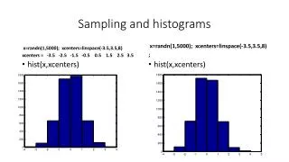
Sampling and histograms x=randn(1,5000); xcenters=linspace(-3.5,3.5,8) xcenters = -3.5 -2.5 -1.5 -0.5 0.5 1.5 2.5 3.5 x=randn(1,5000); xcenters=linspace(-3.5,3.5,8) ; hist(x,xcenters) • hist(x,xcenters)
More boxes • x=randn(1,5000); • hist(x,20) • x=randn(1,5000): • Hist(x,20) )
CDF with only 500 samples z=randn(1,500);[f,x]=ecdf(z); plot(x,f); hold on X=[-4:0.1:4];p=normcdf(X,0,1);plot(X,p,'r'); xlabel('x'); ylabel('normal CDF') Repeat z=randn(1,500);[f,x]=ecdf(z); plot(x,f); three more times
Probability plot • z=randn(1,500); probplot(z) • Repeat (hold off)
Lognormal distribution • Mode (highest point) = • Median (50% of samples) • Mean = • Figure for =0.
Lognormal probability plot z=lognrnd(0,1,1,500);probplot('lognormal',z) probplot(z)
The normalizing effect of averaging z=lognrnd(0,1,100,500); zmean=mean(z); probplot(zmean) mean(zmean') =1.6395 %Exact mean=exp(0.5)= 1.648 std(zmean')= 0.2088 %Original standard deviation=sqrt(exp(1)-1)*exp(1))=2.1612
Fitting a distribution x=randn(20,1)+3; [ecd,xe,elo,eup]=ecdf(x); pd=fitdist(x,'normal') pd = NormalDistribution Normal distribution mu = 2.89147 [2.36524, 3.41771] sigma = 1.1244 [0.855093, 1.64226] xd=linspace(1,8,1000); cdfnorm=normcdf(xd, 2.89147, 1.1244); plot(xe,ecd,'LineWidth',2); hold on; plot(xd,cdfnorm,'r','LineWidth',2); xlabel('x');ylabel('CDF') plot(xe,elo,'LineWidth',1); plot(xe,eup,'LineWidth',1)
Fit lognormal instead pd=fitdist(x,'lognormal') pd = LognormalDistribution Lognormal distribution mu = 0.973822 [0.759473, 1.18817] sigma = 0.457998 [0.348303, 0.668939] cdflogn=logncdf(xd,0.973822,0.45799); hold on; plot(xd,cdflogn,'g','LineWidth',2)
With more points it is clearer Same as before, but with 200 points x=randn(200,1)+3; [ecd,xe,elo,eup]=ecdf(x); pd=fitdist(x,'normal') Normal distribution mu = 3.00311 [2.87373, 3.13248] sigma = 0.927844 [0.844952, 1.02891] pd=fitdist(x,'lognormal') Lognormal distribution mu = 1.04529 [0.996772, 1.09382] sigma = 0.347988 [0.3169, 0.385893]